Organoid Stage integration cluster analysis
Katharina Hembach
9/18/2020
Last updated: 2020-09-21
Checks: 7 0
Knit directory: neural_scRNAseq/
This reproducible R Markdown analysis was created with workflowr (version 1.6.2). The Checks tab describes the reproducibility checks that were applied when the results were created. The Past versions tab lists the development history.
Great! Since the R Markdown file has been committed to the Git repository, you know the exact version of the code that produced these results.
Great job! The global environment was empty. Objects defined in the global environment can affect the analysis in your R Markdown file in unknown ways. For reproduciblity it's best to always run the code in an empty environment.
The command set.seed(20200522) was run prior to running the code in the R Markdown file. Setting a seed ensures that any results that rely on randomness, e.g. subsampling or permutations, are reproducible.
Great job! Recording the operating system, R version, and package versions is critical for reproducibility.
Nice! There were no cached chunks for this analysis, so you can be confident that you successfully produced the results during this run.
Great job! Using relative paths to the files within your workflowr project makes it easier to run your code on other machines.
Great! You are using Git for version control. Tracking code development and connecting the code version to the results is critical for reproducibility.
The results in this page were generated with repository version 6317dad. See the Past versions tab to see a history of the changes made to the R Markdown and HTML files.
Note that you need to be careful to ensure that all relevant files for the analysis have been committed to Git prior to generating the results (you can use wflow_publish or wflow_git_commit). workflowr only checks the R Markdown file, but you know if there are other scripts or data files that it depends on. Below is the status of the Git repository when the results were generated:
Ignored files:
    Ignored:    .DS_Store
    Ignored:    .Rhistory
    Ignored:    .Rproj.user/
    Ignored:    ._.DS_Store
    Ignored:    ._Rplots.pdf
    Ignored:    ._Rplots_largeViz.pdf
    Ignored:    ._Rplots_separate.pdf
    Ignored:    .__workflowr.yml
    Ignored:    ._neural_scRNAseq.Rproj
    Ignored:    analysis/.DS_Store
    Ignored:    analysis/.Rhistory
    Ignored:    analysis/._.DS_Store
    Ignored:    analysis/._01-preprocessing.Rmd
    Ignored:    analysis/._01-preprocessing.html
    Ignored:    analysis/._02.1-SampleQC.Rmd
    Ignored:    analysis/._03-filtering.Rmd
    Ignored:    analysis/._04-clustering.Rmd
    Ignored:    analysis/._04-clustering.knit.md
    Ignored:    analysis/._04.1-cell_cycle.Rmd
    Ignored:    analysis/._05-annotation.Rmd
    Ignored:    analysis/._Lam-0-NSC_no_integration.Rmd
    Ignored:    analysis/._Lam-01-NSC_integration.Rmd
    Ignored:    analysis/._Lam-02-NSC_annotation.Rmd
    Ignored:    analysis/._NSC-1-clustering.Rmd
    Ignored:    analysis/._NSC-2-annotation.Rmd
    Ignored:    analysis/.__site.yml
    Ignored:    analysis/._additional_filtering.Rmd
    Ignored:    analysis/._additional_filtering_clustering.Rmd
    Ignored:    analysis/._index.Rmd
    Ignored:    analysis/._organoid-01-clustering.Rmd
    Ignored:    analysis/._organoid-02-integration.Rmd
    Ignored:    analysis/._organoid-03-cluster_analysis.Rmd
    Ignored:    analysis/._organoid-04-group_integration.Rmd
    Ignored:    analysis/._organoid-04-stage_integration.Rmd
    Ignored:    analysis/._organoid-05-group_integration_cluster_analysis.Rmd
    Ignored:    analysis/._organoid-05-stage_integration_cluster_analysis.Rmd
    Ignored:    analysis/._organoid-06-1-prepare-sce.Rmd
    Ignored:    analysis/._organoid-06-conos-analysis-Seurat.Rmd
    Ignored:    analysis/._organoid-06-conos-analysis-function.Rmd
    Ignored:    analysis/._organoid-06-conos-analysis.Rmd
    Ignored:    analysis/._organoid-06-group-integration-conos-analysis.Rmd
    Ignored:    analysis/._organoid-07-conos-visualization.Rmd
    Ignored:    analysis/._organoid-07-group-integration-conos-visualization.Rmd
    Ignored:    analysis/._organoid-08-conos-comparison.Rmd
    Ignored:    analysis/._organoid-0x-sample_integration.Rmd
    Ignored:    analysis/01-preprocessing_cache/
    Ignored:    analysis/02-1-SampleQC_cache/
    Ignored:    analysis/02-quality_control_cache/
    Ignored:    analysis/02.1-SampleQC_cache/
    Ignored:    analysis/03-filtering_cache/
    Ignored:    analysis/04-clustering_cache/
    Ignored:    analysis/04.1-cell_cycle_cache/
    Ignored:    analysis/05-annotation_cache/
    Ignored:    analysis/Lam-01-NSC_integration_cache/
    Ignored:    analysis/Lam-02-NSC_annotation_cache/
    Ignored:    analysis/NSC-1-clustering_cache/
    Ignored:    analysis/NSC-2-annotation_cache/
    Ignored:    analysis/additional_filtering_cache/
    Ignored:    analysis/additional_filtering_clustering_cache/
    Ignored:    analysis/organoid-01-clustering_cache/
    Ignored:    analysis/organoid-02-integration_cache/
    Ignored:    analysis/organoid-03-cluster_analysis_cache/
    Ignored:    analysis/organoid-04-group_integration_cache/
    Ignored:    analysis/organoid-04-stage_integration_cache/
    Ignored:    analysis/organoid-05-group_integration_cluster_analysis_cache/
    Ignored:    analysis/organoid-06-conos-analysis_cache/
    Ignored:    analysis/organoid-06-conos-analysis_test_cache/
    Ignored:    analysis/organoid-06-group-integration-conos-analysis_cache/
    Ignored:    analysis/organoid-07-conos-visualization_cache/
    Ignored:    analysis/organoid-07-group-integration-conos-visualization_cache/
    Ignored:    analysis/organoid-08-conos-comparison_cache/
    Ignored:    analysis/organoid-0x-sample_integration_cache/
    Ignored:    analysis/sample5_QC_cache/
    Ignored:    data/.DS_Store
    Ignored:    data/._.DS_Store
    Ignored:    data/._.smbdeleteAAA17ed8b4b
    Ignored:    data/._Lam_figure2_markers.R
    Ignored:    data/._known_NSC_markers.R
    Ignored:    data/._known_cell_type_markers.R
    Ignored:    data/._metadata.csv
    Ignored:    data/data_sushi/
    Ignored:    data/filtered_feature_matrices/
    Ignored:    output/.DS_Store
    Ignored:    output/._.DS_Store
    Ignored:    output/._NSC_cluster1_marker_genes.txt
    Ignored:    output/._organoid_integration_cluster1_marker_genes.txt
    Ignored:    output/Lam-01-clustering.rds
    Ignored:    output/NSC_1_clustering.rds
    Ignored:    output/NSC_cluster1_marker_genes.txt
    Ignored:    output/NSC_cluster2_marker_genes.txt
    Ignored:    output/NSC_cluster3_marker_genes.txt
    Ignored:    output/NSC_cluster4_marker_genes.txt
    Ignored:    output/NSC_cluster5_marker_genes.txt
    Ignored:    output/NSC_cluster6_marker_genes.txt
    Ignored:    output/NSC_cluster7_marker_genes.txt
    Ignored:    output/additional_filtering.rds
    Ignored:    output/conos/
    Ignored:    output/conos_organoid-06-conos-analysis.rds
    Ignored:    output/conos_organoid-06-group-integration-conos-analysis.rds
    Ignored:    output/figures/
    Ignored:    output/organoid_integration_cluster10_marker_genes.txt
    Ignored:    output/organoid_integration_cluster11_marker_genes.txt
    Ignored:    output/organoid_integration_cluster12_marker_genes.txt
    Ignored:    output/organoid_integration_cluster13_marker_genes.txt
    Ignored:    output/organoid_integration_cluster14_marker_genes.txt
    Ignored:    output/organoid_integration_cluster15_marker_genes.txt
    Ignored:    output/organoid_integration_cluster16_marker_genes.txt
    Ignored:    output/organoid_integration_cluster17_marker_genes.txt
    Ignored:    output/organoid_integration_cluster1_marker_genes.txt
    Ignored:    output/organoid_integration_cluster2_marker_genes.txt
    Ignored:    output/organoid_integration_cluster3_marker_genes.txt
    Ignored:    output/organoid_integration_cluster4_marker_genes.txt
    Ignored:    output/organoid_integration_cluster5_marker_genes.txt
    Ignored:    output/organoid_integration_cluster6_marker_genes.txt
    Ignored:    output/organoid_integration_cluster7_marker_genes.txt
    Ignored:    output/organoid_integration_cluster8_marker_genes.txt
    Ignored:    output/organoid_integration_cluster9_marker_genes.txt
    Ignored:    output/sce_01_preprocessing.rds
    Ignored:    output/sce_02_quality_control.rds
    Ignored:    output/sce_03_filtering.rds
    Ignored:    output/sce_03_filtering_all_genes.rds
    Ignored:    output/sce_06-1-prepare-sce.rds
    Ignored:    output/sce_organoid-01-clustering.rds
    Ignored:    output/sce_preprocessing.rds
    Ignored:    output/so_04-group_integration.rds
    Ignored:    output/so_04-stage_integration.rds
    Ignored:    output/so_04_1_cell_cycle.rds
    Ignored:    output/so_04_clustering.rds
    Ignored:    output/so_0x-sample_integration.rds
    Ignored:    output/so_additional_filtering_clustering.rds
    Ignored:    output/so_integrated_organoid-02-integration.rds
    Ignored:    output/so_merged_organoid-02-integration.rds
    Ignored:    output/so_organoid-01-clustering.rds
    Ignored:    output/so_sample_organoid-01-clustering.rds

Untracked files:
    Untracked:  Rplots.pdf
    Untracked:  Rplots_largeViz.pdf
    Untracked:  Rplots_separate.pdf
    Untracked:  analysis/Lam-0-NSC_no_integration.Rmd
    Untracked:  analysis/additional_filtering.Rmd
    Untracked:  analysis/additional_filtering_clustering.Rmd
    Untracked:  analysis/organoid-06-conos-analysis-Seurat.Rmd
    Untracked:  analysis/organoid-06-conos-analysis-function.Rmd
    Untracked:  analysis/organoid-07-conos-visualization.Rmd
    Untracked:  analysis/organoid-07-group-integration-conos-visualization.Rmd
    Untracked:  analysis/organoid-08-conos-comparison.Rmd
    Untracked:  analysis/organoid-0x-sample_integration.Rmd
    Untracked:  analysis/sample5_QC.Rmd
    Untracked:  data/Homo_sapiens.GRCh38.98.sorted.gtf
    Untracked:  data/Kanton_et_al/
    Untracked:  data/Lam_et_al/
    Untracked:  scripts/

Unstaged changes:
    Modified:   analysis/05-annotation.Rmd
    Modified:   analysis/Lam-02-NSC_annotation.Rmd
    Modified:   analysis/_site.yml
    Modified:   analysis/organoid-02-integration.Rmd
    Modified:   analysis/organoid-04-group_integration.Rmd
    Modified:   analysis/organoid-06-conos-analysis.Rmd
Note that any generated files, e.g. HTML, png, CSS, etc., are not included in this status report because it is ok for generated content to have uncommitted changes.
These are the previous versions of the repository in which changes were made to the R Markdown (analysis/organoid-05-stage_integration_cluster_analysis.Rmd) and HTML (docs/organoid-05-stage_integration_cluster_analysis.html) files. If you've configured a remote Git repository (see ?wflow_git_remote), click on the hyperlinks in the table below to view the files as they were in that past version.
| File | Version | Author | Date | Message |
|---|---|---|---|---|
| html | 6317dad | khembach | 2020-09-21 | Build site. |
| Rmd | 6d64ace | khembach | 2020-09-21 | fix factor levels |
| html | ff520ae | khembach | 2020-09-20 | Build site. |
| Rmd | f91df7b | khembach | 2020-09-20 | cluster abundances of cell line and stage integration |
Load packages
library(ComplexHeatmap)
library(cowplot)
library(ggplot2)
library(dplyr)
library(muscat)
library(RColorBrewer)
library(Seurat)
library(SingleCellExperiment)
library(scran)
library(stringr)
library(viridis)
Load data & convert to SCE
so <- readRDS(file.path("output", "so_04-stage_integration.rds"))
sce <- as.SingleCellExperiment(so, assay = "RNA")
colData(sce) <- as.data.frame(colData(sce)) %>%
    mutate_if(is.character, as.factor) %>%
    DataFrame(row.names = colnames(sce))
Cluster-sample counts
# set cluster IDs to resolution 0.4 clustering
so <- SetIdent(so, value = "integrated_snn_res.0.4")
so@meta.data$cluster_id <- Idents(so)
sce$cluster_id <- Idents(so)
(n_cells <- table(sce$cluster_id, sce$sample_id))
     1NSC 2NSC 3NC52 4NC52 5NC96 6NC96 h409B2_120d_org1 h409B2_128d_org1
  0    44   38  5980  4810  1611  2512               82               79
  1  3130 3184  1105   952   926  1105               31               48
  10  701  703    37    31     5     2               58               31
  11  436  446   287   254   226   241               50               98
  12    6    9     3     3     0     1               94              104
  13   99  107    41    33    22    19               37                0
  2  1922 1949   111    70    88    35              186               96
  3  1007  993   325   364   388   333              160                2
  4    56   41   374   356    89   155              345              492
  5     0    0    33    27     7     8              141              624
  6    43   34   129   315    90    94              349              585
  7   847  868    79    57    59    33               33               29
  8     0    0    10    32     2     3              699              592
  9    40   36   173   134    25    54              288              340

     h409B2_60d_org1 h409B2_67d_org1 h409B2_EB h409B2_iPSCs
  0              803             731         3            1
  1              126              72       362          690
  10             174             104        54          117
  11             115              72         7           18
  12              95              85         0            0
  13               5               9         0            0
  2              406             316       148          425
  3              156              62        60          123
  4              753             620         0            0
  5              592             315         0            0
  6              216             254        51          192
  7              108              79       170          376
  8              555             363         0            0
  9              488             382         0            1

     h409B2_neuroectoderm h409B2_neuroepithelium h409B2_Org_32d H9_128d_org1
  0                     1                      1            172          486
  1                   300                     79            240            3
  10                   61                     41            148           65
  11                   29                      8             38           36
  12                    0                      0             29          149
  13                    1                      9             11            0
  2                   196                    100            581          118
  3                   107                    143            268            5
  4                     0                      4            489          159
  5                     0                      0             70         1452
  6                    68                     24             40          894
  7                   123                     34            108           23
  8                     0                      0             27          182
  9                     0                      0            195          243

     H9_60d_org1 H9_67d_org1 H9_EB H9_iPSCs H9_neuroectoderm H9_neuroepithelium
  0          551         269    11        5                0                  0
  1           53          37  1065      845              300                106
  10         131         104   144      128              183                 78
  11          31          68    38       50              116                 38
  12         332         153     0        0                0                  0
  13           0          24     0        1                1                  0
  2          275         275   523      415              570                225
  3           12          94   199      132              409                296
  4          670         614     2        1               30                 36
  5         1252         534     0        0                0                  0
  6          219         534    31      314               85                 66
  7          118          69   432      466              172                 65
  8          713        1089     0        0                0                  0
  9          500         443     0        0                5                 10

     H9_Org_32d
  0         222
  1         104
  10        135
  11        181
  12         28
  13          4
  2         327
  3         437
  4         545
  5         131
  6         176
  7          92
  8          15
  9         257
Relative cluster-abundances
fqs <- prop.table(n_cells, margin = 2)
mat <- as.matrix(unclass(fqs))
Heatmap(mat,
    col = rev(brewer.pal(11, "RdGy")[-6]),
    name = "Frequency",
    cluster_rows = FALSE,
    cluster_columns = FALSE,
    row_names_side = "left",
    row_title = "cluster_id",
    column_title = "sample_id",
    column_title_side = "bottom",
    rect_gp = gpar(col = "white"),
    cell_fun = function(i, j, x, y, width, height, fill)
        grid.text(round(mat[j, i] * 100, 2), x = x, y = y,
            gp = gpar(col = "white", fontsize = 10)))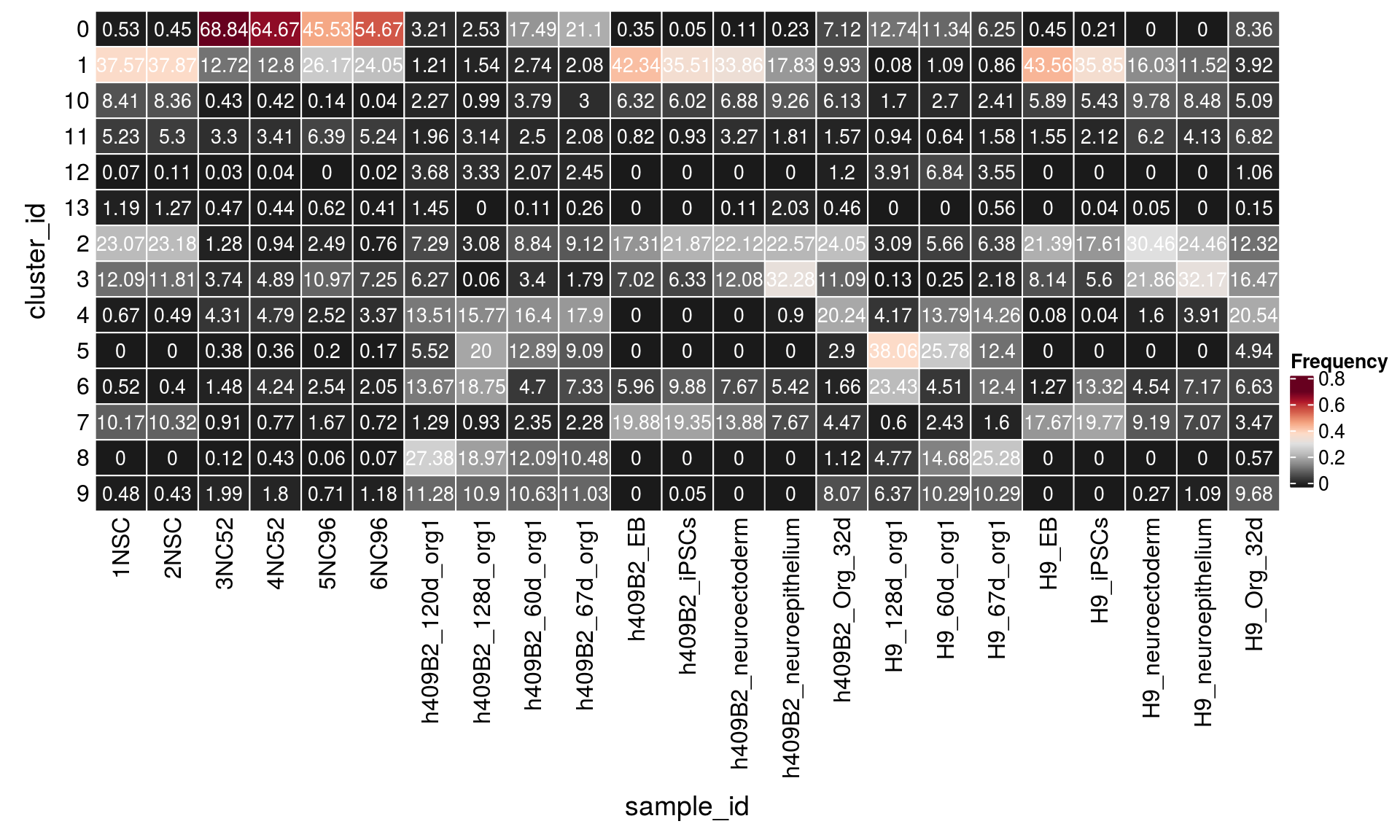
n_cells <- table(sce$sample_id, sce$cluster_id)
fqs <- prop.table(n_cells, margin = 2)
mat <- as.matrix(unclass(fqs))
Heatmap(mat,
    col = rev(brewer.pal(11, "RdGy")[-6]),
    name = "Frequency",
    cluster_rows = FALSE,
    cluster_columns = FALSE,
    row_names_side = "left",
    row_title = "sample_id",
    column_title = "cluster_id",
    column_title_side = "bottom",
    rect_gp = gpar(col = "white"),
    cell_fun = function(i, j, x, y, width, height, fill)
        grid.text(round(mat[j, i] * 100, 2), x = x, y = y,
            gp = gpar(col = "white", fontsize = 10)))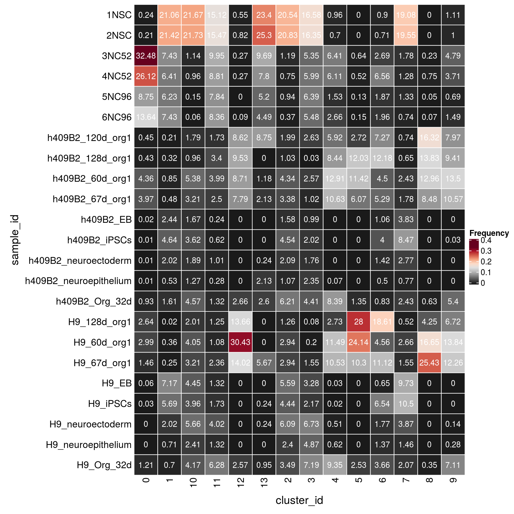
(n_cells_group <- table(sce$cluster_id, sce$group_id))
       P22   D52   D96    H9 409b2
  0     82 10790  4123  1544  1873
  1   6314  2057  2031  2513  1948
  10  1404    68     7   968   788
  11   882   541   467   558   435
  12    15     6     1   662   407
  13   206    74    41    30    72
  2   3871   181   123  2728  2454
  3   2000   689   721  1584  1081
  4     97   730   244  2057  2703
  5      0    60    15  3369  1742
  6     77   444   184  2319  1779
  7   1715   136    92  1437  1060
  8      0    42     5  1999  2236
  9     76   307    79  1458  1694
fqs <- prop.table(n_cells_group, margin = 2)
mat <- as.matrix(unclass(fqs))
Heatmap(mat,
col = rev(brewer.pal(11, "RdGy")[-6]),
name = "Frequency",
cluster_rows = FALSE,
cluster_columns = FALSE,
row_names_side = "left",
row_title = "cluster_id",
column_title = "group_id",
column_title_side = "bottom",
rect_gp = gpar(col = "white"),
cell_fun = function(i, j, x, y, width, height, fill)
grid.text(round(mat[j, i] * 100, 2), x = x, y = y,
gp = gpar(col = "white", fontsize = 10)))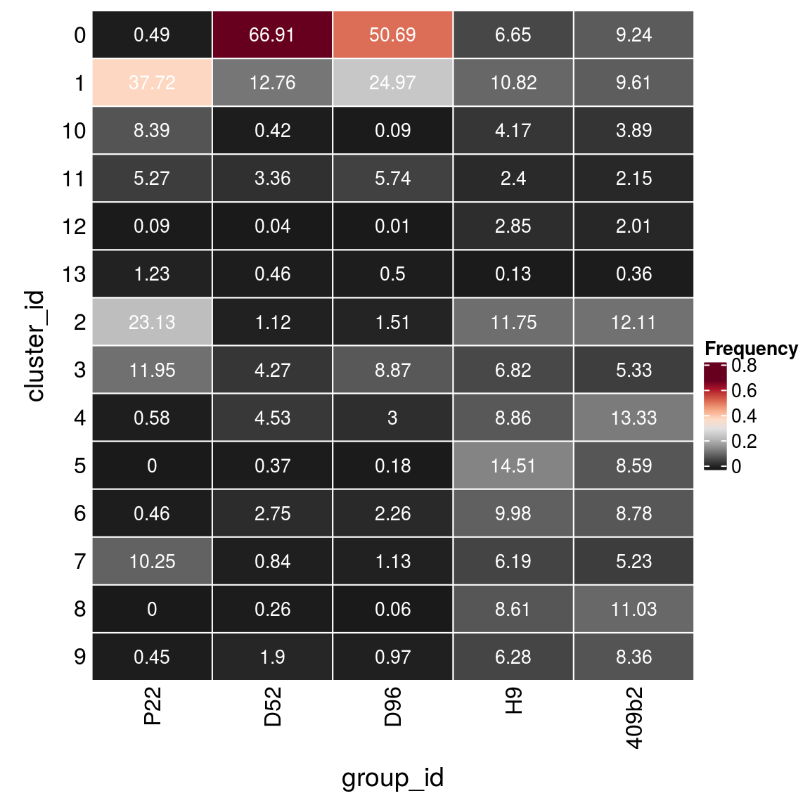
(n_cells_group <- table(sce$cluster_id, sce$Stage))
       P22   D52   D96 iPSCs    EB Neuroectoderm Neuroepithelium Organoid-1M
  0     82 10790  4123     6    14             1               1         394
  1   6314  2057  2031  1535  1427           600             185         344
  10  1404    68     7   245   198           244             119         283
  11   882   541   467    68    45           145              46         219
  12    15     6     1     0     0             0               0          57
  13   206    74    41     1     0             2               9          15
  2   3871   181   123   840   671           766             325         908
  3   2000   689   721   255   259           516             439         705
  4     97   730   244     1     2            30              40        1034
  5      0    60    15     0     0             0               0         201
  6     77   444   184   506    82           153              90         216
  7   1715   136    92   842   602           295              99         200
  8      0    42     5     0     0             0               0          42
  9     76   307    79     1     0             5              10         452

     Organoid-2M Organoid-4M
  0         2354         647
  1          288          82
  10         513         154
  11         286         184
  12         665         347
  13          38          37
  2         1272         400
  3          324         167
  4         2657         996
  5         2693        2217
  6         1223        1828
  7          374          85
  8         2720        1473
  9         1813         871
fqs <- prop.table(n_cells_group, margin = 2)
mat <- as.matrix(unclass(fqs))
Heatmap(mat,
col = rev(brewer.pal(11, "RdGy")[-6]),
name = "Frequency",
cluster_rows = FALSE,
cluster_columns = FALSE,
row_names_side = "left",
row_title = "cluster_id",
column_title = "Stage",
column_title_side = "bottom",
rect_gp = gpar(col = "white"),
cell_fun = function(i, j, x, y, width, height, fill)
grid.text(round(mat[j, i] * 100, 2), x = x, y = y,
gp = gpar(col = "white", fontsize = 10)))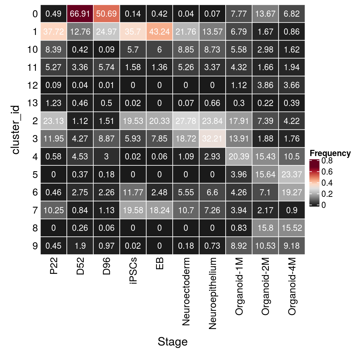
n_cells_lineage <- table(sce$cluster_id, sce$cl_FullLineage)
fqs <- prop.table(n_cells_lineage, margin = 2)
mat <- as.matrix(unclass(fqs))
cn <- colnames(mat)
Heatmap(mat,
    col = rev(brewer.pal(11, "RdGy")[-6]),
    name = "Frequency",
    cluster_rows = FALSE,
    cluster_columns = FALSE,
    show_column_names = FALSE,
    row_names_side = "left",
    row_title = "cluster_id",
    column_title = "cl_FullLineage",
    column_title_side = "bottom",
    rect_gp = gpar(col = "white"),
    cell_fun = function(i, j, x, y, width, height, fill)
        grid.text(round(mat[j, i] * 100, 1), x = x, y = y,
            gp = gpar(col = "white", fontsize = 10)),
    bottom_annotation = HeatmapAnnotation(
      text = anno_text(cn, rot = 80, just = "right")))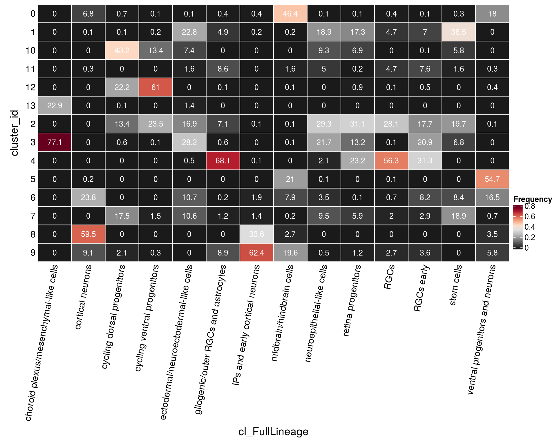
| Version | Author | Date |
|---|---|---|
| 6317dad | khembach | 2020-09-21 |
n_cells_lineage <- table(sce$cl_FullLineage, sce$cluster_id)
fqs <- prop.table(n_cells_lineage, margin = 2)
mat <- as.matrix(unclass(fqs))
Heatmap(mat,
    col = rev(brewer.pal(11, "RdGy")[-6]),
    name = "Frequency",
    cluster_rows = FALSE,
    cluster_columns = FALSE,
    row_names_side = "left",
    row_title = "cl_FullLineage",
    row_names_rot = 10,
    column_title = "cluster_id",
    column_title_side = "bottom",
    rect_gp = gpar(col = "white"),
    cell_fun = function(i, j, x, y, width, height, fill)
        grid.text(round(mat[j, i] * 100, 1), x = x, y = y,
            gp = gpar(col = "white", fontsize = 10)))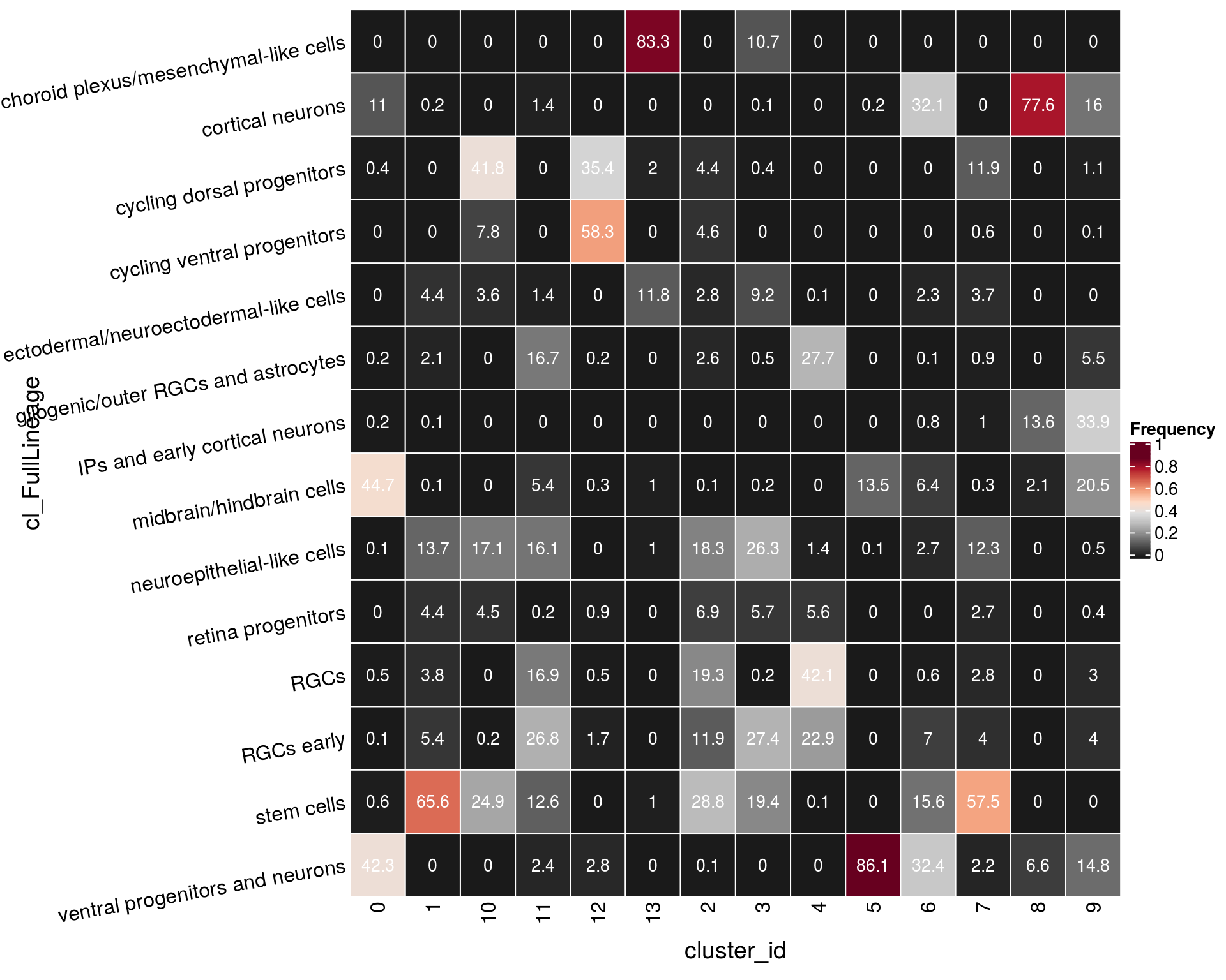
| Version | Author | Date |
|---|---|---|
| 6317dad | khembach | 2020-09-21 |
Evaluation of cluster before and after integration
We evaluate if cells which were together in a cluster before the integration of the organoid cells are still in the same cluster after integration.
## Load the Seurat object from the integrated analysis of our 6 samples
so_before <- readRDS(file.path("output", "so_04_clustering.rds"))
so_before <- SetIdent(so_before, value = "integrated_snn_res.0.4")
so_before@meta.data$cluster_id <- Idents(so_before)
table(so_before@meta.data$cluster_id)
    0     1     2     3     4     5     6     7     8     9    10    11    12
11194  3938  2856  2763  2608  2481  2467  2332  1948  1870  1340  1328  1176
   13    14    15    16
  976   915   488   317
## subset to our cells
cs <- which(so@meta.data$integration_group %in% c("P22", "D52", "D96"))
sub <- subset(so, cells = cs)
table(sub@meta.data$cluster_id)
    0     1    10    11    12    13     2     3     4     5     6     7     8
14995 10402  1479  1890    22   321  4175  3410  1071    75   705  1943    47
    9
  462
## join the cluster_ids from both clustering runs
before <- data.frame(cell = colnames(so_before),
cluster_before = so_before@meta.data[,c("cluster_id")])
after <- data.frame(cell = colnames(sub),
cluster_after = sub@meta.data[,c("cluster_id")])
clusters <- before %>% full_join(after)
## check if cells from the same cluster are still in the same cluster
(n_clusters <- table(clusters$cluster_after, clusters$cluster_before))
        0    1    2    3    4    5    6    7    8    9   10   11   12   13   14
  0    70 3703    0    1    0 2129 2280 2189    1 1716    4  105 1057  924  816
  1  5978   87    1  639 1972   48   83   36  863   69  160  174   51   22   16
  10   99    1 1345    4    0    1    0    1    0    0   26    0    0    0    0
  11  100   18    0   31   38   26   17   34   61   20  871  619   15    4   33
  12    0    0   21    1    0    0    0    0    0    0    0    0    0    0    0
  13    0    0    0   57    0    0    0    0    0    0    0    0    0    0    0
  2  2281   34 1297  220   21   24   12    2   49   15  164   22   18    7    6
  3  1029    7   12 1628  125    1    2    1  456    7    9   71    9    0    0
  4    99    0    0   85  417    0    0    0  457    0   11    1    0    0    0
  5     0    7    0    0    0   43   10   12    0    2    0    0    0    1    0
  6    48   22    0   22   18   47   27   47   37   23   25  320   16   15   37
  7  1446   48  180   48   17   25   34    6   24   17   70   15    4    1    2
  8     0   11    0    0    0   23    2    4    0    1    0    0    4    2    0
  9    44    0    0   27    0  114    0    0    0    0    0    1    2    0    5

       15   16
  0     0    0
  1   202    1
  10    1    1
  11    3    0
  12    0    0
  13    0  264
  2     2    1
  3     3   50
  4     1    0
  5     0    0
  6     1    0
  7     6    0
  8     0    0
  9   269    0
fqs <- prop.table(n_clusters, margin = 2)
mat <- as.matrix(unclass(fqs))
Heatmap(mat,
col = rev(brewer.pal(11, "RdGy")[-6]),
name = "Frequency",
cluster_rows = FALSE,
cluster_columns = FALSE,
row_names_side = "left",
row_title = "clusters after organoid integration",
column_title = "clusters before organoid integration",
column_title_side = "bottom",
rect_gp = gpar(col = "white"),
cell_fun = function(i, j, x, y, width, height, fill)
grid.text(round(mat[j, i] * 100, 2), x = x, y = y,
gp = gpar(col = "white", fontsize = 8)))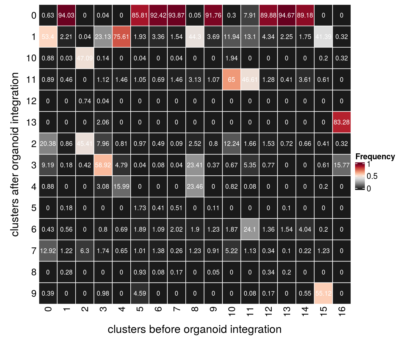
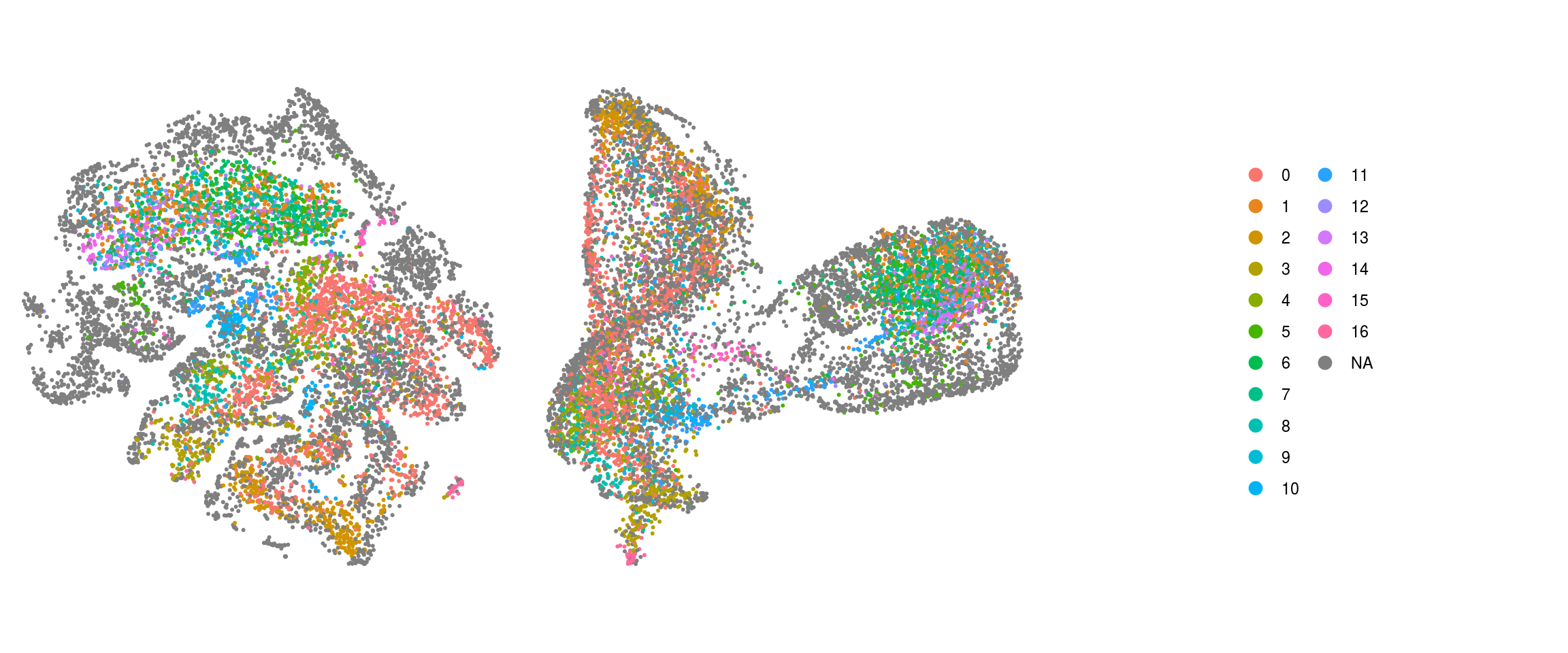
## add the old cluster identities to the Seurat object
so@meta.data$cluster_id_before <- so_before@meta.data$cluster_id[
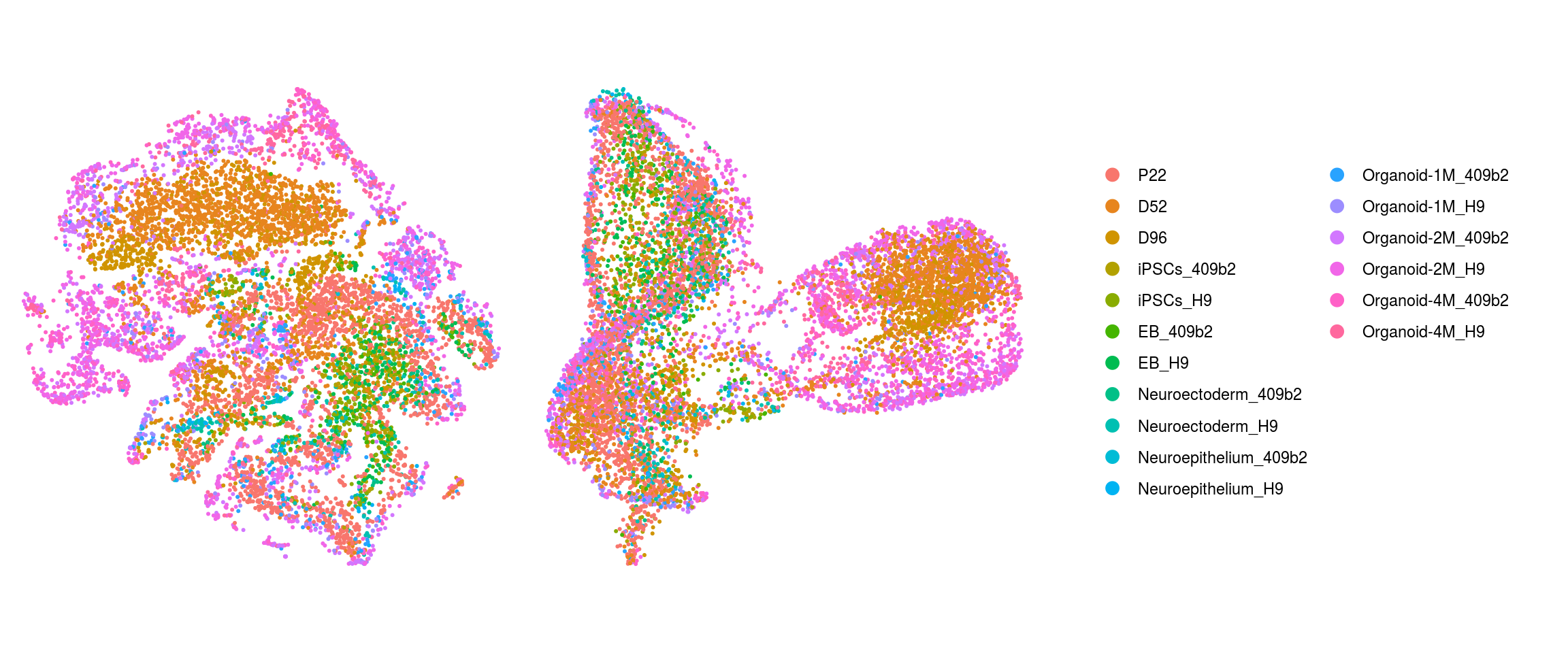
match(colnames(so), colnames(so_before))]Dimension reduction plots
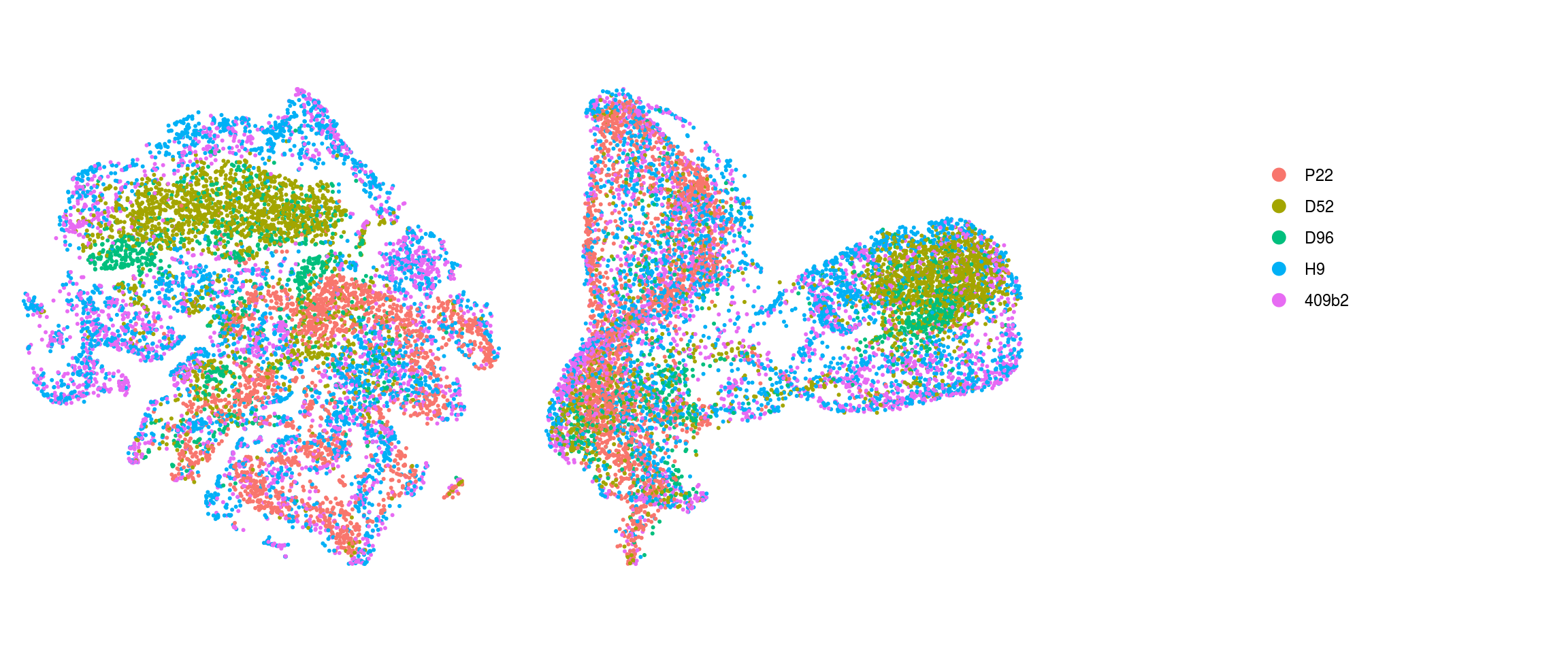
so$integration_group <- factor(so$integration_group,
levels = c("P22", "D52", "D96", "iPSCs_409b2", "iPSCs_H9", "EB_409b2",
"EB_H9", "Neuroectoderm_409b2", "Neuroectoderm_H9",
"Neuroepithelium_409b2", "Neuroepithelium_H9",
"Organoid-1M_409b2", "Organoid-1M_H9", "Organoid-2M_409b2",
"Organoid-2M_H9", "Organoid-4M_409b2", "Organoid-4M_H9"))
cs <- sample(colnames(so), 10e3)
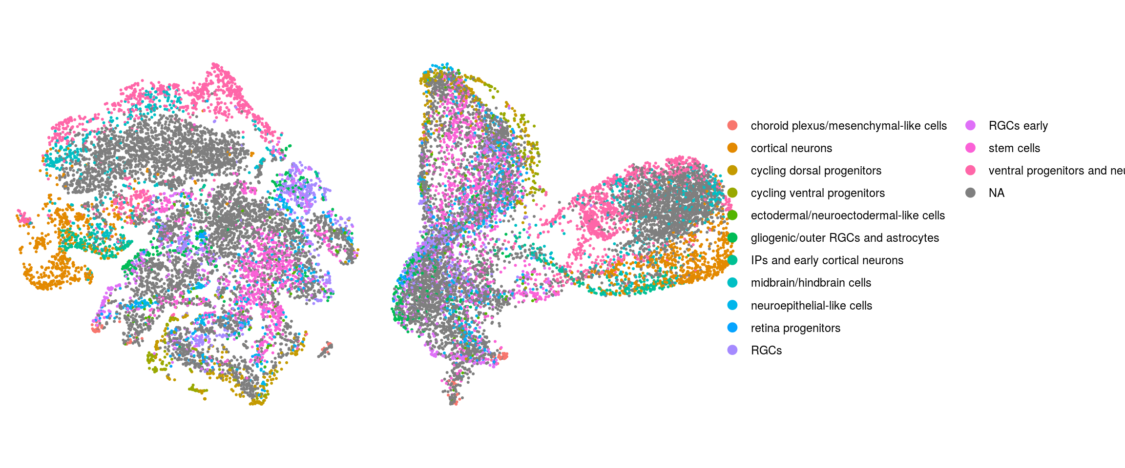
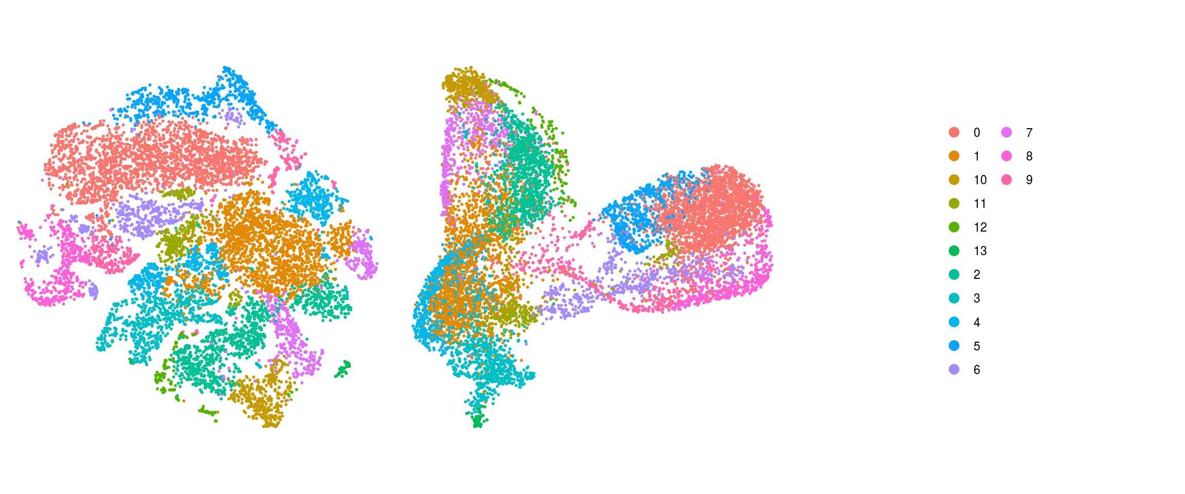
.plot_dr <- function(so, dr, id)
DimPlot(so, cells = cs, group.by = id, reduction = dr, pt.size = 0.4) +
guides(col = guide_legend(nrow = 11,
override.aes = list(size = 3, alpha = 1))) +
theme_void() + theme(aspect.ratio = 1)
ids <- c("integration_group", "group_id", "cl_FullLineage", "cluster_id",
"cluster_id_before")
for (id in ids) {
cat("## ", id, "\n")
p1 <- .plot_dr(so, "tsne", id)
lgd <- get_legend(p1)
p1 <- p1 + theme(legend.position = "none")
p2 <- .plot_dr(so, "umap", id) + theme(legend.position = "none")
ps <- plot_grid(plotlist = list(p1, p2), nrow = 1)
p <- plot_grid(ps, lgd, nrow = 1, rel_widths = c(1, 0.5))
print(p)
cat("\n\n")
}
Find markers using scran
We identify candidate marker genes for each cluster.
scran_markers <- findMarkers(sce,
    groups = sce$cluster_id, block = sce$sample_id,
    direction = "up", lfc = 2, full.stats = TRUE)
Heatmap of mean marker-exprs. by cluster
We aggregate the cells to pseudobulks and plot the average expression of the candidate marker genes in each of the clusters.
gs <- lapply(scran_markers, function(u) rownames(u)[u$Top == 1])
## candidate cluster markers
lapply(gs, function(x) str_split(x, pattern = "\\.", simplify = TRUE)[,2])
$`0`
[1] "SAMD11" "STMN2" "RTN1" "SEZ6L2" "MT-CO3"
$`1`
[1] "SAMD11" "VIM" "CKB" "MT-CO1"
$`10`
[1] "CENPF" "HMGB2" "VIM" "UBE2C"
$`11`
[1] "SAMD11" "PTN" "VIM" "SLC3A2" "CKB"
$`12`
[1] "HES6" "HMGB2" "HIST1H4C" "CKB"
$`13`
[1] "S100A11" "COL3A1" "LGALS1"
$`2`
[1] "SAMD11" "HIST1H4C" "VIM" "CKB" "MT-CO3"
$`3`
[1] "SAMD11" "SPARC" "PTN" "CLU" "VIM" "MT-CO1"
$`4`
[1] "SAMD11" "C1orf61" "FABP7" "VIM" "TTYH1"
$`5`
[1] "SAMD11" "STMN2" "MT-ATP6" "DLX6-AS1"
$`6`
[1] "SAMD11" "IGFBP2" "TUBB2B" "STMN2" "RTN1" "ALDOA"
$`7`
[1] "SAMD11" "HMGB2" "PTTG1" "VIM" "CKB" "MT-CO1"
$`8`
[1] "STMN2" "NFIB" "NEUROD2" "MT-CO3"
$`9`
[1] "HES6" "SOX4" "STMN2" "CKB" sub <- sce[unique(unlist(gs)), ]
pbs <- aggregateData(sub, assay = "logcounts", by = "cluster_id", fun = "mean")
mat <- t(muscat:::.scale(assay(pbs)))
## remove the Ensembl ID from the gene names
colnames(mat) <- str_split(colnames(mat), pattern = "\\.", simplify = TRUE)[,2]
Heatmap(mat,
name = "scaled avg.\nexpression",
col = viridis(10),
cluster_rows = FALSE,
cluster_columns = FALSE,
row_names_side = "left",
row_title = "cluster_id",
rect_gp = gpar(col = "white"))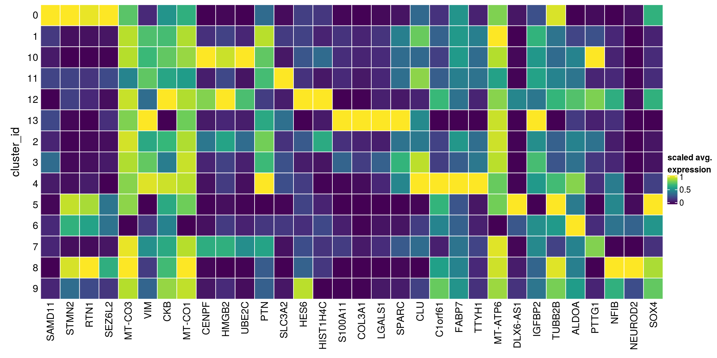
We write tables with the top marker genes per cluster.
gs2 <- lapply(scran_markers, function(u) u[u$Top %in% 1:3,])
for (i in seq_along(gs2)) {
  write.table(x = gs2[[i]] %>% as.data.frame %>%
                dplyr::mutate(gene = rownames(gs2[[i]])) %>%
                dplyr::relocate(gene),
              file =  file.path("output",
                                paste0("organoid_integration_cluster", i, "_marker_genes.txt")),
              sep = "\t", quote = FALSE, row.names = FALSE)
}
Heatmap including marker genes of rank 2 and 3.
gs <- lapply(scran_markers, function(u) rownames(u)[u$Top %in% 1:3])
## candidate cluster markers
lapply(gs, function(x) str_split(x, pattern = "\\.", simplify = TRUE)[,2])
$`0`
[1] "SAMD11" "STMN2" "RTN1" "SEZ6L2" "MT-CO3" "NOC2L" "STMN1"
[8] "GAP43" "DCX" "MT-ATP6" "KLHL17" "NSG1" "STMN4" "MT-CO2"
[15] "HMP19"
$`1`
[1] "SAMD11" "VIM" "CKB" "MT-CO1" "NOC2L" "SOX2" "PTN" "CLU"
[9] "TTYH1" "MT-CO2" "KLHL17" "FABP7" "PTPRZ1" "MT-CO3"
$`10`
[1] "CENPF" "HMGB2" "VIM" "UBE2C" "SAMD11" "CCNB1" "PTTG1"
[8] "TOP2A" "NOC2L" "CKB" "ARL6IP1"
$`11`
[1] "SAMD11" "PTN" "VIM" "SLC3A2" "CKB" "NOC2L"
[7] "CLU" "EIF4EBP1" "MT-CO1" "KLHL17" "ENO1" "SOX2"
[13] "TUBB2B" "BNIP3" "DDIT3" "TTYH1" "MT-CO2"
$`12`
[1] "HES6" "HMGB2" "HIST1H4C" "CKB" "HMGN2" "SOX4" "TUBA1B"
[8] "CDK1" "TOP2A"
$`13`
[1] "S100A11" "COL3A1" "LGALS1" "COL1A1" "TAGLN" "TPM1"
$`2`
[1] "SAMD11" "HIST1H4C" "VIM" "CKB" "MT-CO3" "NOC2L"
[7] "HMGB2" "PTN" "MT-CO1" "KLHL17" "SOX2" "FABP7"
[13] "MT-CO2" "KIAA0101"
$`3`
[1] "SAMD11" "SPARC" "PTN" "CLU" "VIM" "MT-CO1" "NOC2L" "HES1"
[9] "CKB" "MT-CO2" "KLHL17" "METRN" "MT-CO3" "TTR"
$`4`
[1] "SAMD11" "C1orf61" "FABP7" "VIM" "TTYH1" "NOC2L" "SOX2"
[8] "PTN" "CKB" "KLHL17"
$`5`
[1] "SAMD11" "STMN2" "MT-ATP6" "DLX6-AS1" "NOC2L" "SOX4"
[7] "RTN1" "DCX" "MT-CO3" "DLX5" "KLHL17" "MLLT11"
[13] "CD24" "MT-CYB" "DLX2"
$`6`
[1] "SAMD11" "IGFBP2" "TUBB2B" "STMN2" "RTN1" "ALDOA" "NOC2L" "ENO1"
[9] "CKB" "DCX" "KLHL17" "GPM6A" "SOX4" "BEX1"
$`7`
[1] "SAMD11" "HMGB2" "PTTG1" "VIM" "CKB" "MT-CO1" "NOC2L" "CENPF"
[9] "PTN" "MT-CO2" "KLHL17" "FABP7" "UBE2S" "MT-CO3"
$`8`
[1] "STMN2" "NFIB" "NEUROD2" "MT-CO3" "NEUROD6" "CSRP2" "RTN1"
[8] "MT-ATP6" "SAMD11" "SOX4" "DCX" "MT-CO1"
$`9`
[1] "HES6" "SOX4" "STMN2" "CKB" "SAMD11" "MLLT11" "FABP7" "VIM"
[9] "MT-CO3" "NOC2L" "SOX11" "MT-CO2"sub <- sce[unique(unlist(gs)), ]
pbs <- aggregateData(sub, assay = "logcounts", by = "cluster_id", fun = "mean")
mat <- t(muscat:::.scale(assay(pbs)))
## remove the Ensembl ID from the gene names
colnames(mat) <- str_split(colnames(mat), pattern = "\\.", simplify = TRUE)[,2]
Heatmap(mat,
name = "scaled avg.\nexpression",
col = viridis(10),
cluster_rows = FALSE,
cluster_columns = FALSE,
row_names_side = "left",
row_title = "cluster_id",
rect_gp = gpar(col = "white"))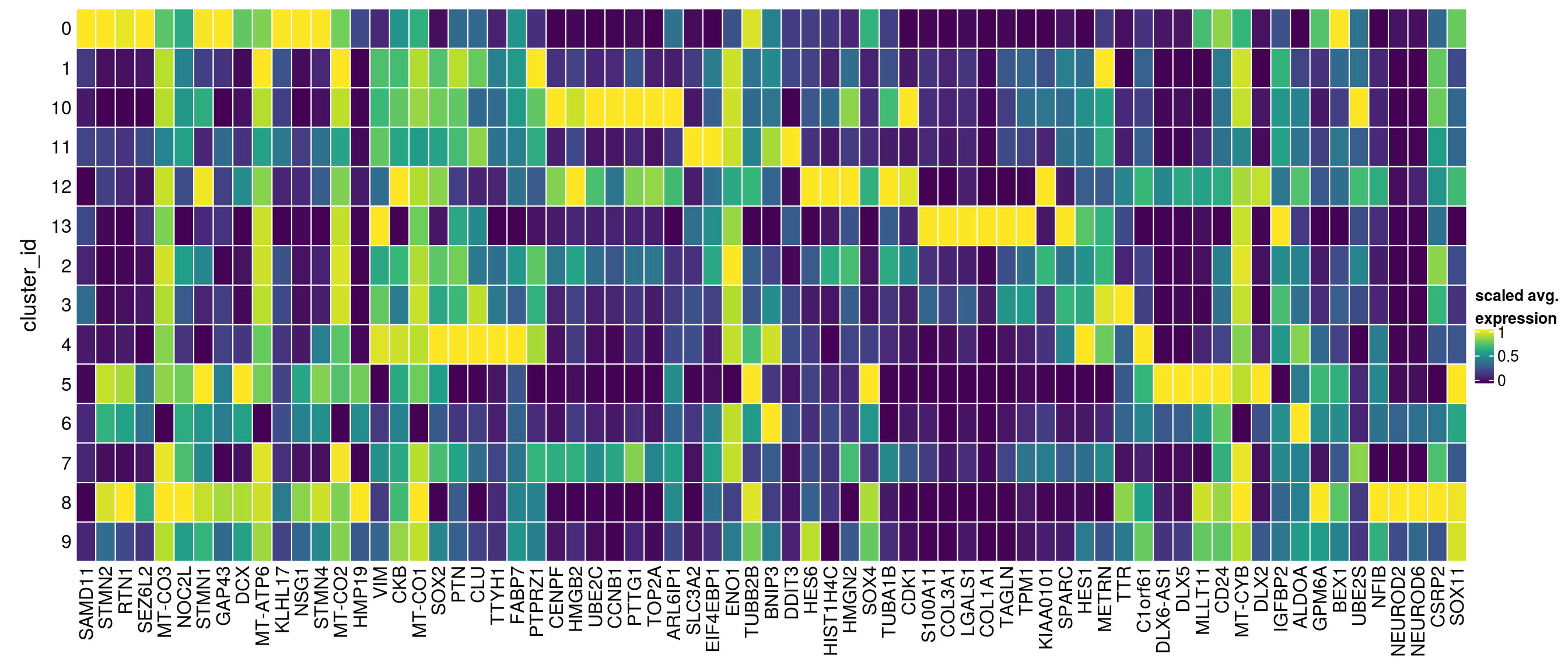
| Version | Author | Date |
|---|---|---|
| 6317dad | khembach | 2020-09-21 |
sessionInfo()R version 4.0.0 (2020-04-24)
Platform: x86_64-pc-linux-gnu (64-bit)
Running under: Ubuntu 16.04.6 LTS
Matrix products: default
BLAS: /usr/local/R/R-4.0.0/lib/libRblas.so
LAPACK: /usr/local/R/R-4.0.0/lib/libRlapack.so
locale:
[1] LC_CTYPE=en_US.UTF-8 LC_NUMERIC=C
[3] LC_TIME=en_US.UTF-8 LC_COLLATE=en_US.UTF-8
[5] LC_MONETARY=en_US.UTF-8 LC_MESSAGES=en_US.UTF-8
[7] LC_PAPER=en_US.UTF-8 LC_NAME=C
[9] LC_ADDRESS=C LC_TELEPHONE=C
[11] LC_MEASUREMENT=en_US.UTF-8 LC_IDENTIFICATION=C
attached base packages:
[1] parallel stats4 grid stats graphics grDevices utils
[8] datasets methods base
other attached packages:
[1] viridis_0.5.1 viridisLite_0.3.0
[3] stringr_1.4.0 scran_1.16.0
[5] SingleCellExperiment_1.10.1 SummarizedExperiment_1.18.1
[7] DelayedArray_0.14.0 matrixStats_0.56.0
[9] Biobase_2.48.0 GenomicRanges_1.40.0
[11] GenomeInfoDb_1.24.2 IRanges_2.22.2
[13] S4Vectors_0.26.1 BiocGenerics_0.34.0
[15] Seurat_3.1.5 RColorBrewer_1.1-2
[17] muscat_1.2.1 dplyr_1.0.2
[19] ggplot2_3.3.2 cowplot_1.0.0
[21] ComplexHeatmap_2.4.2 workflowr_1.6.2
loaded via a namespace (and not attached):
[1] backports_1.1.9 circlize_0.4.10
[3] blme_1.0-4 igraph_1.2.5
[5] plyr_1.8.6 lazyeval_0.2.2
[7] TMB_1.7.16 splines_4.0.0
[9] BiocParallel_1.22.0 listenv_0.8.0
[11] scater_1.16.2 digest_0.6.25
[13] foreach_1.5.0 htmltools_0.5.0
[15] gdata_2.18.0 lmerTest_3.1-2
[17] magrittr_1.5 memoise_1.1.0
[19] cluster_2.1.0 doParallel_1.0.15
[21] ROCR_1.0-11 limma_3.44.3
[23] globals_0.12.5 annotate_1.66.0
[25] prettyunits_1.1.1 colorspace_1.4-1
[27] rappdirs_0.3.1 ggrepel_0.8.2
[29] blob_1.2.1 xfun_0.15
[31] jsonlite_1.7.0 crayon_1.3.4
[33] RCurl_1.98-1.2 genefilter_1.70.0
[35] lme4_1.1-23 zoo_1.8-8
[37] ape_5.4 survival_3.2-3
[39] iterators_1.0.12 glue_1.4.2
[41] gtable_0.3.0 zlibbioc_1.34.0
[43] XVector_0.28.0 leiden_0.3.3
[45] GetoptLong_1.0.1 BiocSingular_1.4.0
[47] future.apply_1.6.0 shape_1.4.4
[49] scales_1.1.1 DBI_1.1.0
[51] edgeR_3.30.3 Rcpp_1.0.5
[53] xtable_1.8-4 progress_1.2.2
[55] clue_0.3-57 dqrng_0.2.1
[57] reticulate_1.16 bit_1.1-15.2
[59] rsvd_1.0.3 tsne_0.1-3
[61] htmlwidgets_1.5.1 httr_1.4.1
[63] gplots_3.0.4 ellipsis_0.3.1
[65] ica_1.0-2 farver_2.0.3
[67] pkgconfig_2.0.3 XML_3.99-0.4
[69] uwot_0.1.8 locfit_1.5-9.4
[71] labeling_0.3 tidyselect_1.1.0
[73] rlang_0.4.7 reshape2_1.4.4
[75] later_1.1.0.1 AnnotationDbi_1.50.1
[77] munsell_0.5.0 tools_4.0.0
[79] generics_0.0.2 RSQLite_2.2.0
[81] ggridges_0.5.2 evaluate_0.14
[83] yaml_2.2.1 knitr_1.29
[85] bit64_0.9-7 fs_1.4.2
[87] fitdistrplus_1.1-1 caTools_1.18.0
[89] RANN_2.6.1 purrr_0.3.4
[91] pbapply_1.4-2 future_1.17.0
[93] nlme_3.1-148 whisker_0.4
[95] pbkrtest_0.4-8.6 compiler_4.0.0
[97] plotly_4.9.2.1 beeswarm_0.2.3
[99] png_0.1-7 variancePartition_1.18.2
[101] tibble_3.0.3 statmod_1.4.34
[103] geneplotter_1.66.0 stringi_1.4.6
[105] lattice_0.20-41 Matrix_1.2-18
[107] nloptr_1.2.2.2 vctrs_0.3.4
[109] pillar_1.4.6 lifecycle_0.2.0
[111] lmtest_0.9-37 GlobalOptions_0.1.2
[113] RcppAnnoy_0.0.16 BiocNeighbors_1.6.0
[115] data.table_1.12.8 bitops_1.0-6
[117] irlba_2.3.3 patchwork_1.0.1
[119] httpuv_1.5.4 colorRamps_2.3
[121] R6_2.4.1 promises_1.1.1
[123] KernSmooth_2.23-17 gridExtra_2.3
[125] vipor_0.4.5 codetools_0.2-16
[127] boot_1.3-25 MASS_7.3-51.6
[129] gtools_3.8.2 DESeq2_1.28.1
[131] rprojroot_1.3-2 rjson_0.2.20
[133] withr_2.2.0 sctransform_0.2.1
[135] GenomeInfoDbData_1.2.3 hms_0.5.3
[137] tidyr_1.1.0 glmmTMB_1.0.2.1
[139] minqa_1.2.4 rmarkdown_2.3
[141] DelayedMatrixStats_1.10.1 Rtsne_0.15
[143] git2r_0.27.1 numDeriv_2016.8-1.1
[145] ggbeeswarm_0.6.0