Cluster analysis of group integrated cells
Katharina Hembach
8/26/2020
Last updated: 2020-09-07
Checks: 7 0
Knit directory: neural_scRNAseq/
This reproducible R Markdown analysis was created with workflowr (version 1.6.2). The Checks tab describes the reproducibility checks that were applied when the results were created. The Past versions tab lists the development history.
Great! Since the R Markdown file has been committed to the Git repository, you know the exact version of the code that produced these results.
Great job! The global environment was empty. Objects defined in the global environment can affect the analysis in your R Markdown file in unknown ways. For reproduciblity it's best to always run the code in an empty environment.
The command set.seed(20200522) was run prior to running the code in the R Markdown file. Setting a seed ensures that any results that rely on randomness, e.g. subsampling or permutations, are reproducible.
Great job! Recording the operating system, R version, and package versions is critical for reproducibility.
Nice! There were no cached chunks for this analysis, so you can be confident that you successfully produced the results during this run.
Great job! Using relative paths to the files within your workflowr project makes it easier to run your code on other machines.
Great! You are using Git for version control. Tracking code development and connecting the code version to the results is critical for reproducibility.
The results in this page were generated with repository version f4c394f. See the Past versions tab to see a history of the changes made to the R Markdown and HTML files.
Note that you need to be careful to ensure that all relevant files for the analysis have been committed to Git prior to generating the results (you can use wflow_publish or wflow_git_commit). workflowr only checks the R Markdown file, but you know if there are other scripts or data files that it depends on. Below is the status of the Git repository when the results were generated:
Ignored files:
    Ignored:    .DS_Store
    Ignored:    .Rhistory
    Ignored:    .Rproj.user/
    Ignored:    ._.DS_Store
    Ignored:    ._Rplots.pdf
    Ignored:    ._Rplots_separate.pdf
    Ignored:    .__workflowr.yml
    Ignored:    ._neural_scRNAseq.Rproj
    Ignored:    analysis/.DS_Store
    Ignored:    analysis/.Rhistory
    Ignored:    analysis/._.DS_Store
    Ignored:    analysis/._01-preprocessing.Rmd
    Ignored:    analysis/._01-preprocessing.html
    Ignored:    analysis/._02.1-SampleQC.Rmd
    Ignored:    analysis/._03-filtering.Rmd
    Ignored:    analysis/._04-clustering.Rmd
    Ignored:    analysis/._04-clustering.knit.md
    Ignored:    analysis/._04.1-cell_cycle.Rmd
    Ignored:    analysis/._05-annotation.Rmd
    Ignored:    analysis/._Lam-0-NSC_no_integration.Rmd
    Ignored:    analysis/._Lam-01-NSC_integration.Rmd
    Ignored:    analysis/._Lam-02-NSC_annotation.Rmd
    Ignored:    analysis/._NSC-1-clustering.Rmd
    Ignored:    analysis/._NSC-2-annotation.Rmd
    Ignored:    analysis/.__site.yml
    Ignored:    analysis/._additional_filtering.Rmd
    Ignored:    analysis/._additional_filtering_clustering.Rmd
    Ignored:    analysis/._index.Rmd
    Ignored:    analysis/._organoid-01-clustering.Rmd
    Ignored:    analysis/._organoid-02-integration.Rmd
    Ignored:    analysis/._organoid-03-cluster_analysis.Rmd
    Ignored:    analysis/._organoid-04-group_integration.Rmd
    Ignored:    analysis/._organoid-05-group_integration_cluster_analysis.Rmd
    Ignored:    analysis/._organoid-06-1-conos-analysis.Rmd
    Ignored:    analysis/._organoid-06-conos-analysis.Rmd
    Ignored:    analysis/01-preprocessing_cache/
    Ignored:    analysis/02-1-SampleQC_cache/
    Ignored:    analysis/02-quality_control_cache/
    Ignored:    analysis/02.1-SampleQC_cache/
    Ignored:    analysis/03-filtering_cache/
    Ignored:    analysis/04-clustering_cache/
    Ignored:    analysis/04.1-cell_cycle_cache/
    Ignored:    analysis/05-annotation_cache/
    Ignored:    analysis/Lam-01-NSC_integration_cache/
    Ignored:    analysis/Lam-02-NSC_annotation_cache/
    Ignored:    analysis/NSC-1-clustering_cache/
    Ignored:    analysis/NSC-2-annotation_cache/
    Ignored:    analysis/additional_filtering_cache/
    Ignored:    analysis/additional_filtering_clustering_cache/
    Ignored:    analysis/organoid-01-clustering_cache/
    Ignored:    analysis/organoid-02-integration_cache/
    Ignored:    analysis/organoid-03-cluster_analysis_cache/
    Ignored:    analysis/organoid-04-group_integration_cache/
    Ignored:    analysis/sample5_QC_cache/
    Ignored:    data/.DS_Store
    Ignored:    data/._.DS_Store
    Ignored:    data/._.smbdeleteAAA17ed8b4b
    Ignored:    data/._Lam_figure2_markers.R
    Ignored:    data/._known_NSC_markers.R
    Ignored:    data/._known_cell_type_markers.R
    Ignored:    data/._metadata.csv
    Ignored:    data/data_sushi/
    Ignored:    data/filtered_feature_matrices/
    Ignored:    output/.DS_Store
    Ignored:    output/._.DS_Store
    Ignored:    output/._NSC_cluster1_marker_genes.txt
    Ignored:    output/._organoid_integration_cluster1_marker_genes.txt
    Ignored:    output/Lam-01-clustering.rds
    Ignored:    output/NSC_1_clustering.rds
    Ignored:    output/NSC_cluster1_marker_genes.txt
    Ignored:    output/NSC_cluster2_marker_genes.txt
    Ignored:    output/NSC_cluster3_marker_genes.txt
    Ignored:    output/NSC_cluster4_marker_genes.txt
    Ignored:    output/NSC_cluster5_marker_genes.txt
    Ignored:    output/NSC_cluster6_marker_genes.txt
    Ignored:    output/NSC_cluster7_marker_genes.txt
    Ignored:    output/additional_filtering.rds
    Ignored:    output/figures/
    Ignored:    output/organoid_integration_cluster10_marker_genes.txt
    Ignored:    output/organoid_integration_cluster11_marker_genes.txt
    Ignored:    output/organoid_integration_cluster12_marker_genes.txt
    Ignored:    output/organoid_integration_cluster13_marker_genes.txt
    Ignored:    output/organoid_integration_cluster14_marker_genes.txt
    Ignored:    output/organoid_integration_cluster15_marker_genes.txt
    Ignored:    output/organoid_integration_cluster16_marker_genes.txt
    Ignored:    output/organoid_integration_cluster17_marker_genes.txt
    Ignored:    output/organoid_integration_cluster1_marker_genes.txt
    Ignored:    output/organoid_integration_cluster2_marker_genes.txt
    Ignored:    output/organoid_integration_cluster3_marker_genes.txt
    Ignored:    output/organoid_integration_cluster4_marker_genes.txt
    Ignored:    output/organoid_integration_cluster5_marker_genes.txt
    Ignored:    output/organoid_integration_cluster6_marker_genes.txt
    Ignored:    output/organoid_integration_cluster7_marker_genes.txt
    Ignored:    output/organoid_integration_cluster8_marker_genes.txt
    Ignored:    output/organoid_integration_cluster9_marker_genes.txt
    Ignored:    output/sce_01_preprocessing.rds
    Ignored:    output/sce_02_quality_control.rds
    Ignored:    output/sce_03_filtering.rds
    Ignored:    output/sce_organoid-01-clustering.rds
    Ignored:    output/sce_preprocessing.rds
    Ignored:    output/so_04-group_integration.rds
    Ignored:    output/so_04_1_cell_cycle.rds
    Ignored:    output/so_04_clustering.rds
    Ignored:    output/so_additional_filtering_clustering.rds
    Ignored:    output/so_integrated_organoid-02-integration.rds
    Ignored:    output/so_merged_organoid-02-integration.rds
    Ignored:    output/so_organoid-01-clustering.rds
    Ignored:    output/so_sample_organoid-01-clustering.rds

Untracked files:
    Untracked:  Rplots.pdf
    Untracked:  Rplots_separate.pdf
    Untracked:  analysis/Lam-0-NSC_no_integration.Rmd
    Untracked:  analysis/additional_filtering.Rmd
    Untracked:  analysis/additional_filtering_clustering.Rmd
    Untracked:  analysis/organoid-06-1-conos-analysis.Rmd
    Untracked:  analysis/organoid-06-conos-analysis.Rmd
    Untracked:  analysis/sample5_QC.Rmd
    Untracked:  data/Homo_sapiens.GRCh38.98.sorted.gtf
    Untracked:  data/Kanton_et_al/
    Untracked:  data/Lam_et_al/
    Untracked:  scripts/

Unstaged changes:
    Modified:   analysis/Lam-02-NSC_annotation.Rmd
    Modified:   analysis/_site.yml
    Modified:   analysis/organoid-02-integration.Rmd
Note that any generated files, e.g. HTML, png, CSS, etc., are not included in this status report because it is ok for generated content to have uncommitted changes.
These are the previous versions of the repository in which changes were made to the R Markdown (analysis/organoid-05-group_integration_cluster_analysis.Rmd) and HTML (docs/organoid-05-group_integration_cluster_analysis.html) files. If you've configured a remote Git repository (see ?wflow_git_remote), click on the hyperlinks in the table below to view the files as they were in that past version.
| File | Version | Author | Date | Message |
|---|---|---|---|---|
| Rmd | f4c394f | khembach | 2020-09-07 | fix tabset |
| html | 48fb578 | khembach | 2020-09-07 | Build site. |
| Rmd | b6abb6f | khembach | 2020-09-07 | add marker genes, heatmap, comparison with clusters before organoid |
| html | 1e1dcab | khembach | 2020-09-03 | Build site. |
| Rmd | e72cff9 | khembach | 2020-09-03 | add sample abundance plot |
| html | b93b07d | khembach | 2020-09-02 | Build site. |
| Rmd | 043115f | khembach | 2020-09-02 | group organoid integration cluster abundances |
Load packages
library(ComplexHeatmap)
library(cowplot)
library(ggplot2)
library(dplyr)
library(muscat)
library(RColorBrewer)
library(Seurat)
library(SingleCellExperiment)
library(scran)
library(stringr)
library(viridis)
Load data & convert to SCE
so <- readRDS(file.path("output", "so_04-group_integration.rds"))
sce <- as.SingleCellExperiment(so, assay = "RNA")
colData(sce) <- as.data.frame(colData(sce)) %>%
    mutate_if(is.character, as.factor) %>%
    DataFrame(row.names = colnames(sce))
Cluster-sample counts
# set cluster IDs to resolution 0.4 clustering
so <- SetIdent(so, value = "integrated_snn_res.0.4")
so@meta.data$cluster_id <- Idents(so)
sce$cluster_id <- Idents(so)
(n_cells <- table(sce$cluster_id, sce$sample_id))
     1NSC 2NSC 3NC52 4NC52 5NC96 6NC96   H9 409b2
  0    17   16  5165  4290  1352  2047 2722  2391
  1  4357 4307   281   193   421    49   64    78
  2    11   12  1307  1316   802  1321 1787  2672
  3  3111 3232    30    17     7     2  414   395
  4     0    0   393   337    90    96 2483  3335
  5     1    0     7    31     6     7 3656  1244
  6    35   22   780   522   360   565  475  1016
  7     0    0     0     0     0     0 2017  1708
  8     0    0     1     0     0     0 2409   817
  9     4    1     9     9    12     4 1866  1174
  10    3    3    28    12     7     8 1619  1351
  11    5    7    39    40     3     6 1472  1382
  12  539  553   270   232   271   247  215   358
  13    0    2     0     0     0     1  811  1149
  14    1    3   191   162    51   101  666   754
  15  244  245   186   277   156   141  127   170
  16    3    5     0     0     0     0  423   278
Relative cluster-abundances
fqs <- prop.table(n_cells, margin = 2)
mat <- as.matrix(unclass(fqs))
Heatmap(mat,
    col = rev(brewer.pal(11, "RdGy")[-6]),
    name = "Frequency",
    cluster_rows = FALSE,
    cluster_columns = FALSE,
    row_names_side = "left",
    row_title = "cluster_id",
    column_title = "sample_id",
    column_title_side = "bottom",
    rect_gp = gpar(col = "white"),
    cell_fun = function(i, j, x, y, width, height, fill)
        grid.text(round(mat[j, i] * 100, 2), x = x, y = y,
            gp = gpar(col = "white", fontsize = 10)))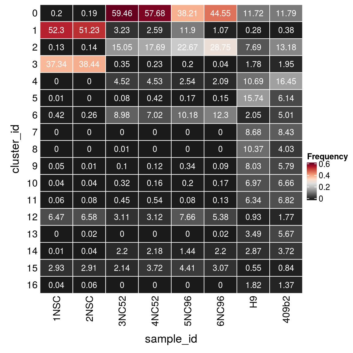
| Version | Author | Date |
|---|---|---|
| b93b07d | khembach | 2020-09-02 |
n_cells <- table(sce$sample_id, sce$cluster_id)
fqs <- prop.table(n_cells, margin = 2)
mat <- as.matrix(unclass(fqs))
Heatmap(mat,
    col = rev(brewer.pal(11, "RdGy")[-6]),
    name = "Frequency",
    cluster_rows = FALSE,
    cluster_columns = FALSE,
    row_names_side = "left",
    row_title = "sample_id",
    column_title = "cluster_id",
    column_title_side = "bottom",
    rect_gp = gpar(col = "white"),
    cell_fun = function(i, j, x, y, width, height, fill)
        grid.text(round(mat[j, i] * 100, 2), x = x, y = y,
            gp = gpar(col = "white", fontsize = 10)))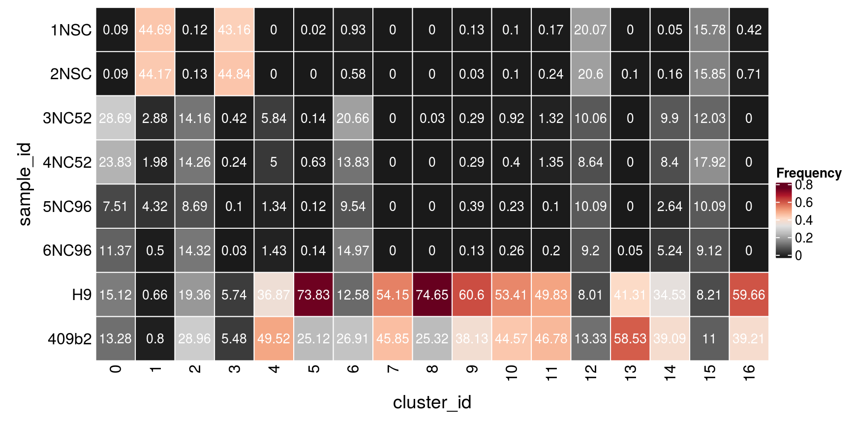
(n_cells_group <- table(sce$cluster_id, sce$group_id))
      P22  D52  D96 iPSCs   EB Neuroectoderm Neuroepithelium Organoid-1M
  0    33 9455 3399     0    0             0               0         266
  1  8664  474  470     0    0             0               1          18
  2    23 2623 2123     0    0             0               0           5
  3  6343   47    9     8   16             4              29         297
  4     0  730  186     0    0             0               0           0
  5     1   38   13     0    0             0               2          67
  6    57 1302  925     0    0             1               0         753
  7     0    0    0  3656   16            53               0           0
  8     0    1    0    16 3203             7               0           0
  9     5   18   16    19    6          2635             375           5
  10    6   40   15     0    0             1               7        2350
  11   12   79    9     0    0             0               0          49
  12 1092  502  518     0    0             2               7         161
  13    2    0    1    11   15             9             913        1012
  14    4  353  152     0    0             0               0           9
  15  489  463  297     0    0             4               4          78
  16    8    0    0   590   44            41              25           0

     Organoid-2M Organoid-4M
  0         3878         969
  1          102          21
  2         3139        1315
  3          398          57
  4         3553        2265
  5         1476        3355
  6          735           2
  7            0           0
  8            0           0
  9            0           0
  10         607           5
  11        1955         850
  12         241         162
  13           0           0
  14         983         428
  15         152          59
  16           1           0
fqs <- prop.table(n_cells_group, margin = 2)
mat <- as.matrix(unclass(fqs))
Heatmap(mat,
col = rev(brewer.pal(11, "RdGy")[-6]),
name = "Frequency",
cluster_rows = FALSE,
cluster_columns = FALSE,
row_names_side = "left",
row_title = "cluster_id",
column_title = "group_id",
column_title_side = "bottom",
rect_gp = gpar(col = "white"),
cell_fun = function(i, j, x, y, width, height, fill)
grid.text(round(mat[j, i] * 100, 2), x = x, y = y,
gp = gpar(col = "white", fontsize = 10)))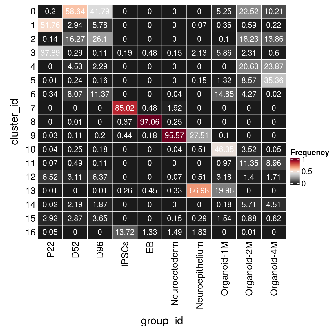
n_cells_lineage <- table(sce$cluster_id, sce$cl_FullLineage)
fqs <- prop.table(n_cells_lineage, margin = 2)
mat <- as.matrix(unclass(fqs))
cn <- colnames(mat)
Heatmap(mat,
    col = rev(brewer.pal(11, "RdGy")[-6]),
    name = "Frequency",
    cluster_rows = FALSE,
    cluster_columns = FALSE,
    show_column_names = FALSE,
    row_names_side = "left",
    row_title = "cluster_id",
    column_title = "cl_FullLineage",
    column_title_side = "bottom",
    rect_gp = gpar(col = "white"),
    cell_fun = function(i, j, x, y, width, height, fill)
        grid.text(round(mat[j, i] * 100, 1), x = x, y = y,
            gp = gpar(col = "white", fontsize = 10)),
    bottom_annotation = HeatmapAnnotation(
      text = anno_text(cn, rot = 80, just = "right")))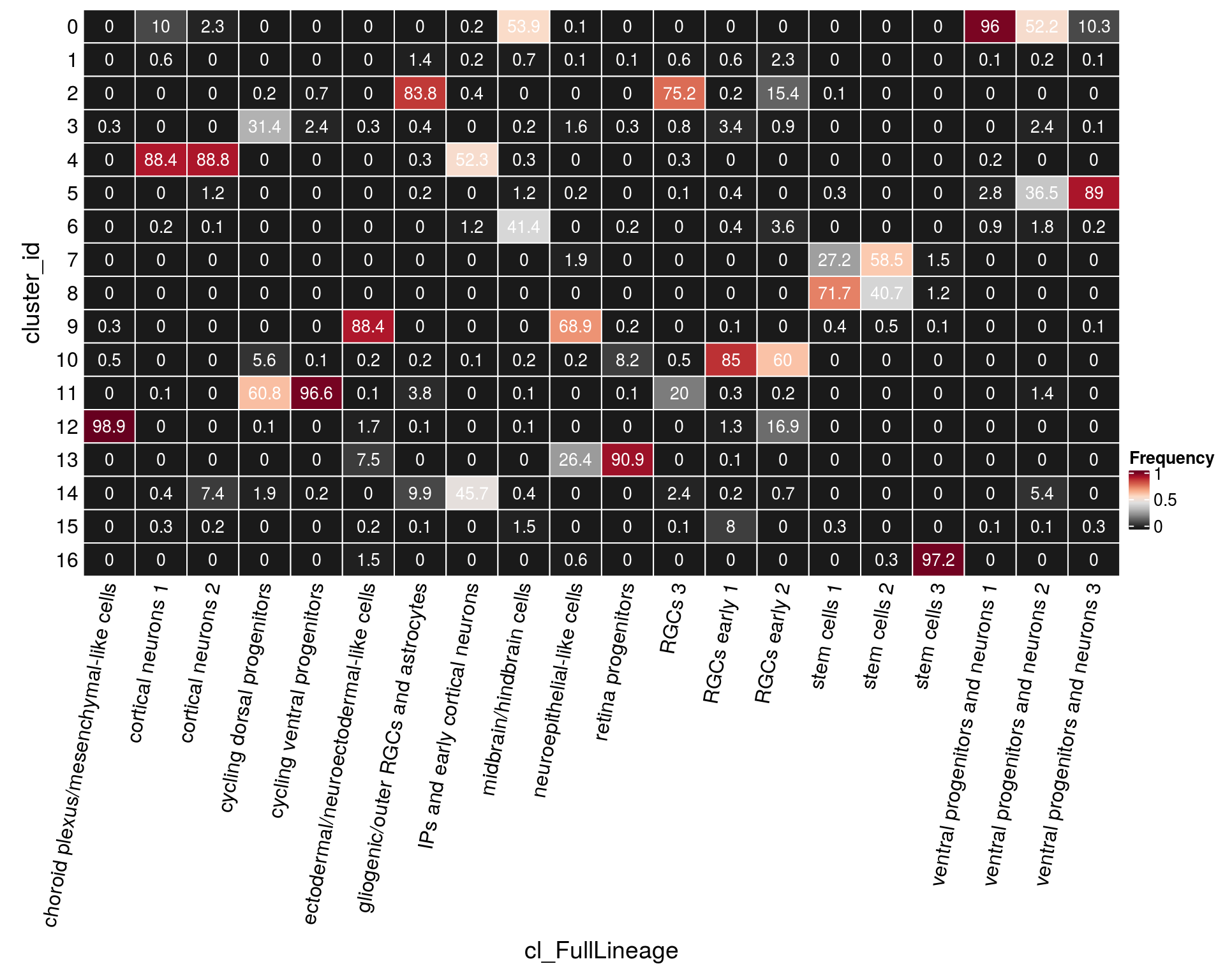
| Version | Author | Date |
|---|---|---|
| 1e1dcab | khembach | 2020-09-03 |
n_cells_lineage <- table(sce$cl_FullLineage, sce$cluster_id)
fqs <- prop.table(n_cells_lineage, margin = 2)
mat <- as.matrix(unclass(fqs))
Heatmap(mat,
    col = rev(brewer.pal(11, "RdGy")[-6]),
    name = "Frequency",
    cluster_rows = FALSE,
    cluster_columns = FALSE,
    row_names_side = "left",
    row_title = "cl_FullLineage",
    row_names_rot = 10,
    column_title = "cluster_id",
    column_title_side = "bottom",
    rect_gp = gpar(col = "white"),
    cell_fun = function(i, j, x, y, width, height, fill)
        grid.text(round(mat[j, i] * 100, 1), x = x, y = y,
            gp = gpar(col = "white", fontsize = 10)))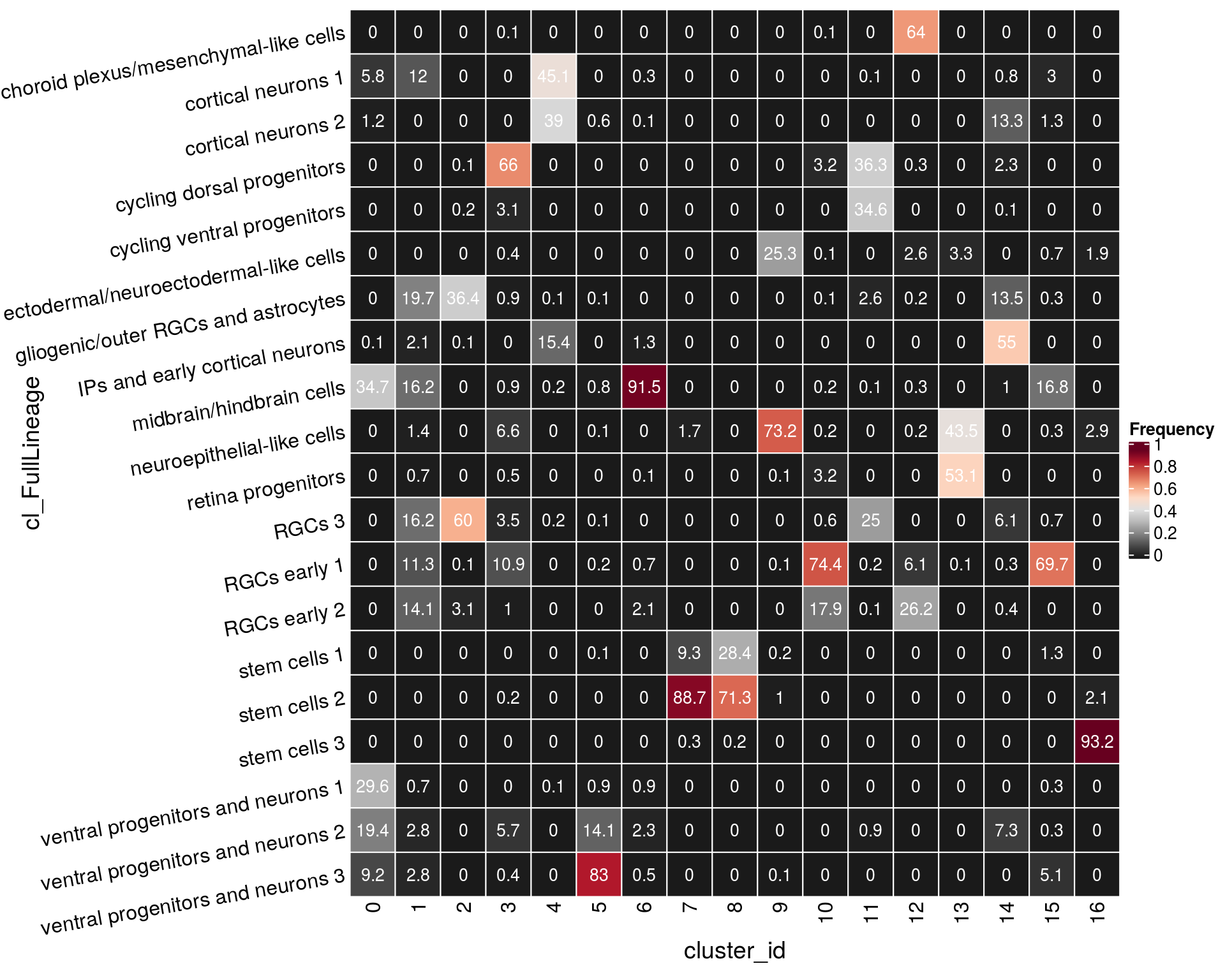
| Version | Author | Date |
|---|---|---|
| 1e1dcab | khembach | 2020-09-03 |
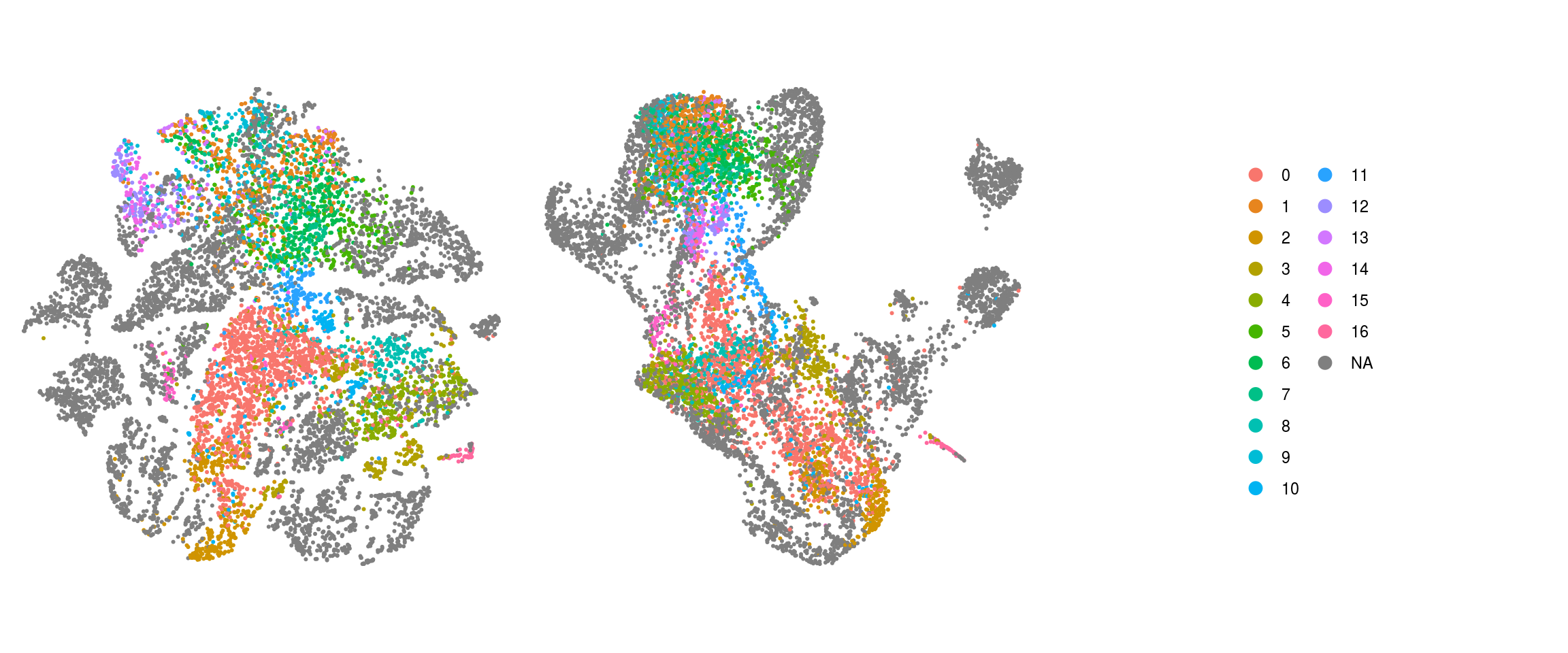
Evaluation of cluster before and after integration
We evaluate if cells which were together in a cluster before the integration of the organoid cells are still in the same cluster after integration.
## Load the Seurat object from our NSC analysis
so_before <- readRDS(file.path("output", "so_04_clustering.rds"))
so_before <- SetIdent(so_before, value = "integrated_snn_res.0.4")
so_before@meta.data$cluster_id <- Idents(so_before)
table(so_before@meta.data$cluster_id)
    0     1     2     3     4     5     6     7     8     9    10    11    12
11194  3938  2856  2763  2608  2481  2467  2332  1948  1870  1340  1328  1176
   13    14    15    16
  976   915   488   317
## subset to our cells
cs <- which(so@meta.data$integration_group %in% c("P22", "D52", "D96"))
sub <- subset(so, cells = cs)
table(sub@meta.data$cluster_id)
    0     1     2     3     4     5     6     7     8     9    10    11    12
12887  9608  4769  6399   916    52  2284     0     1    39    61   100  2112
   13    14    15    16
    3   509  1249     8
## join the cluster_ids from both clustering runs
before <- data.frame(cell = colnames(so_before),
cluster_before = so_before@meta.data[,c("cluster_id")])
after <- data.frame(cell = colnames(sub),
cluster_after = sub@meta.data[,c("cluster_id")])
clusters <- before %>% full_join(after)
## check if cells from the same cluster are still in the same cluster
(n_clusters <- table(clusters$cluster_after, clusters$cluster_before))
        0    1    2    3    4    5    6    7    8    9   10   11   12   13   14
  0    31 3854    0    1    0 1560 2378 2296    0 1624    1  128  125  840   48
  1  7371   32   13  514   70    7   17    5  530   46  761  110   44   26   10
  2   367    0    4  313 2518    0    0    0 1262    0  256    8    0    0    0
  3  3126    0 2727  284    3    0    0    0   14    0  236    3    2    0    0
  4     0    4    0    0    0  836   57   10    0    1    0    8    0    0    0
  5     1    7    0    1    0    6    3   10    0    2    0   18    1    2    0
  6    34   33    0    0    0   34    0    0    0  189    2    7 1002  104  850
  7     0    0    0    0    0    0    0    0    0    0    0    0    0    0    0
  8     0    0    0    1    0    0    0    0    0    0    0    0    0    0    0
  9     2    0    2    7    0    0    0    0    0    0   26    2    0    0    0
  10   11    0    3   10    2    0    0    0   17    0   13    3    0    0    0
  11    1    0   96    3    0    0    0    0    0    0    0    0    0    0    0
  12  176    0    9 1531    2    0    0    0   66    0    5    6    0    0    0
  13    0    0    2    1    0    0    0    0    0    0    0    0    0    0    0
  14   17    0    0   79    6   29    0    0   18    0    0    1    0    0    2
  15   51    8    0   17    6    9   12   11   41    8   40 1034    2    4    5
  16    6    0    0    1    1    0    0    0    0    0    0    0    0    0    0

       15   16
  0     1    0
  1    52    0
  2    41    0
  3     4    0
  4     0    0
  5     1    0
  6    29    0
  7     0    0
  8     0    0
  9     0    0
  10    2    0
  11    0    0
  12    0  317
  13    0    0
  14  357    0
  15    1    0
  16    0    0
fqs <- prop.table(n_clusters, margin = 2)
mat <- as.matrix(unclass(fqs))
Heatmap(mat,
col = rev(brewer.pal(11, "RdGy")[-6]),
name = "Frequency",
cluster_rows = FALSE,
cluster_columns = FALSE,
row_names_side = "left",
row_title = "clusters after organoid integration",
column_title = "clusters before organoid integration",
column_title_side = "bottom",
rect_gp = gpar(col = "white"),
cell_fun = function(i, j, x, y, width, height, fill)
grid.text(round(mat[j, i] * 100, 2), x = x, y = y,
gp = gpar(col = "white", fontsize = 8)))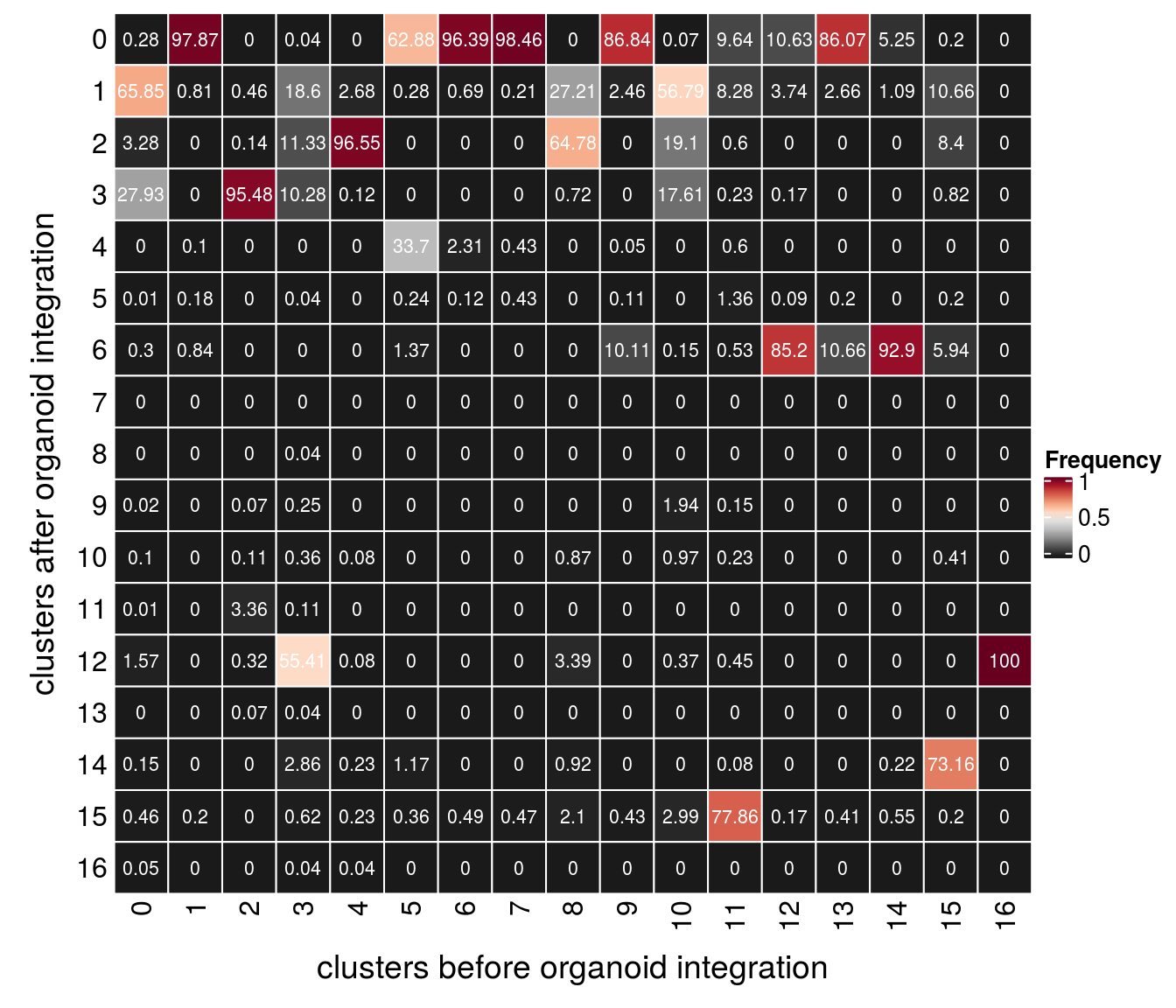
| Version | Author | Date |
|---|---|---|
| 48fb578 | khembach | 2020-09-07 |
## add the old cluster identities to the Seurat object
so@meta.data$cluster_id_before <- so_before@meta.data$cluster_id[
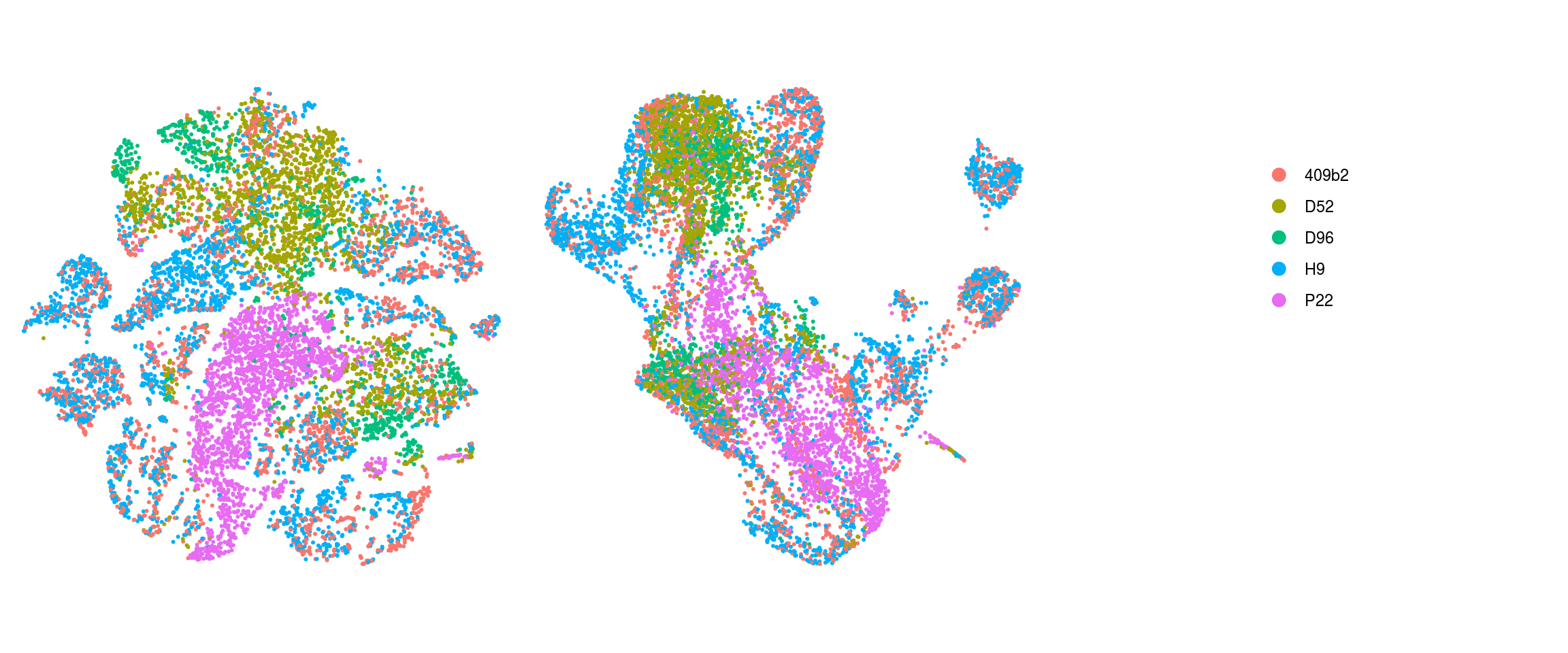
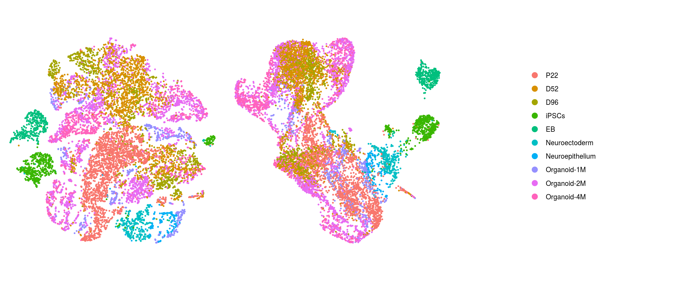
match(colnames(so), colnames(so_before))]Dimension reduction plots
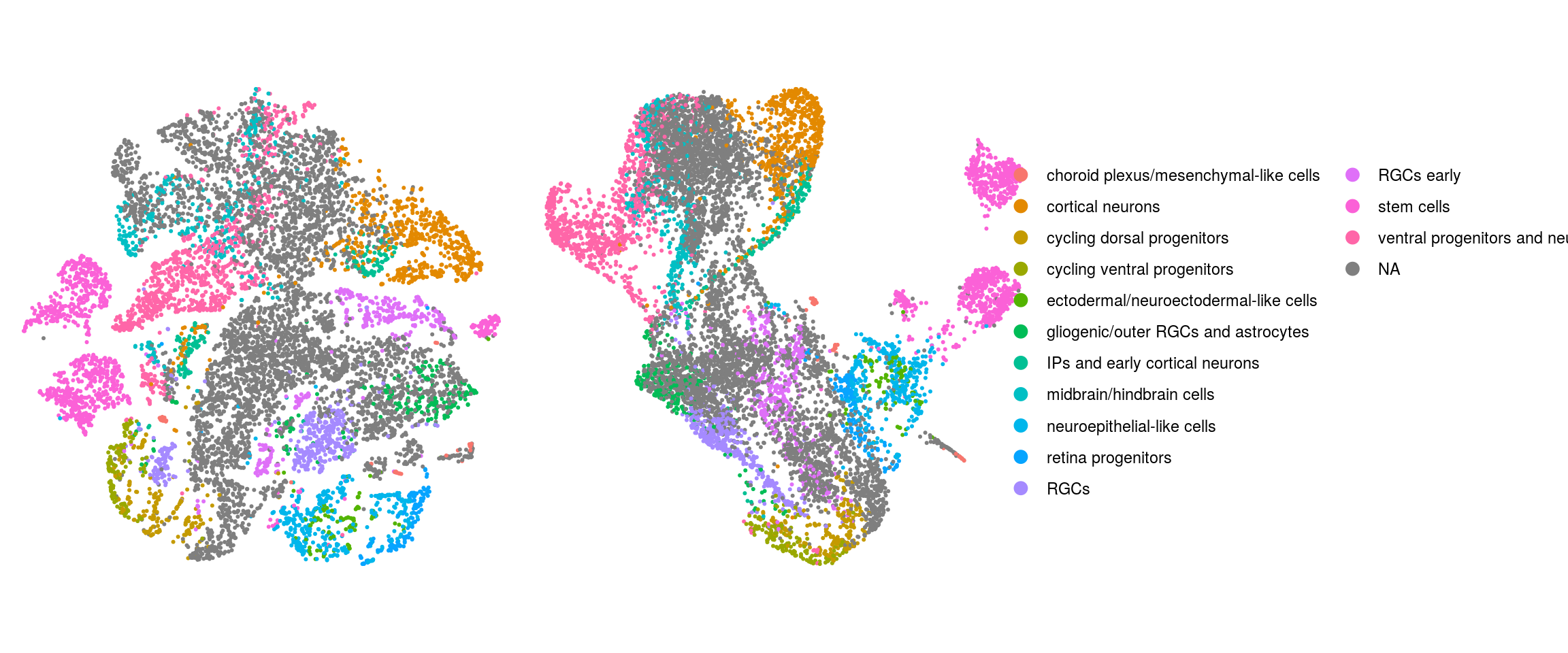
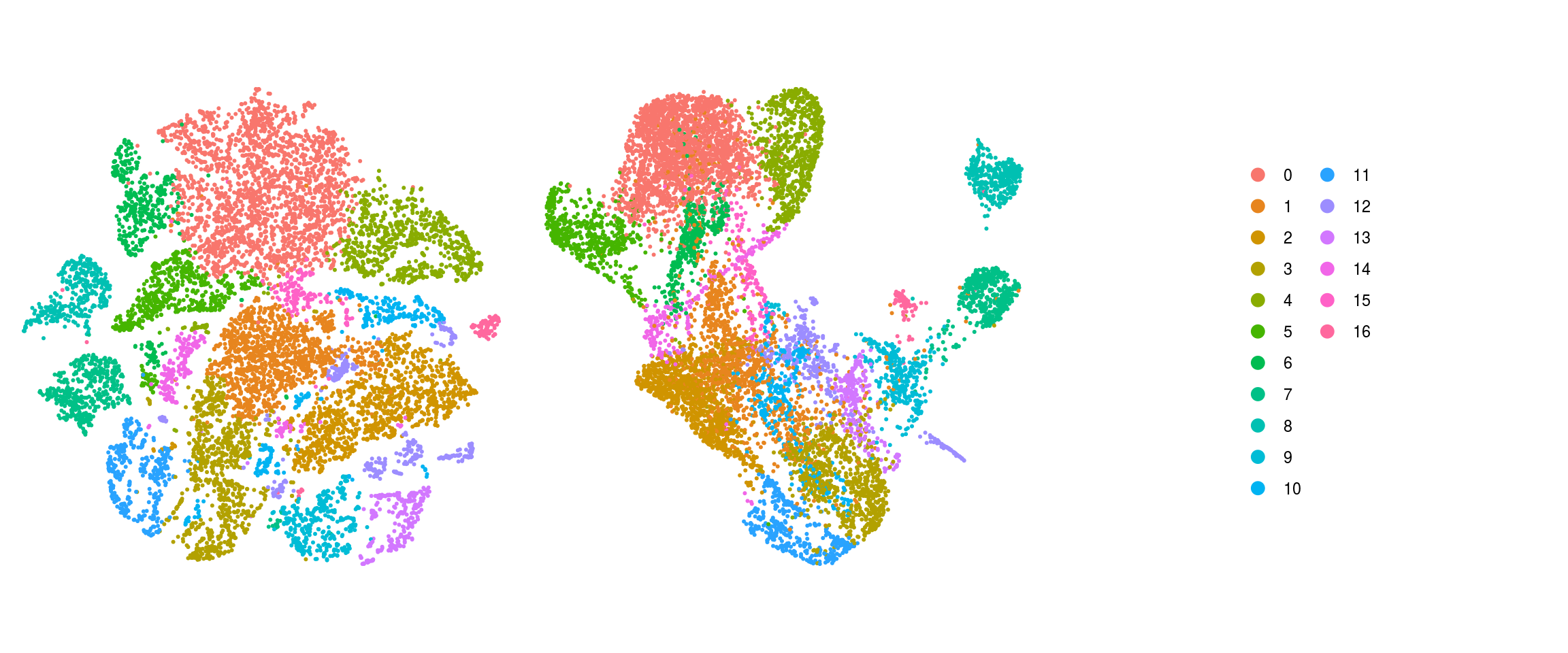
## merge the lineage labels of identical cell types
so$cl_FullLineage_merged <- as.factor(so$cl_FullLineage)
levels(so$cl_FullLineage_merged) <- c("choroid plexus/mesenchymal-like cells",
               "cortical neurons", "cortical neurons",
               "cycling dorsal progenitors", "cycling ventral progenitors",
               "ectodermal/neuroectodermal-like cells",
               "gliogenic/outer RGCs and astrocytes",
               "IPs and early cortical neurons", "midbrain/hindbrain cells",
               "neuroepithelial-like cells", "retina progenitors", "RGCs",
               "RGCs early", "RGCs early", "stem cells", "stem cells",
               "stem cells", "ventral progenitors and neurons",
               "ventral progenitors and neurons",
               "ventral progenitors and neurons")

cs <- sample(colnames(so), 10e3)
.plot_dr <- function(so, dr, id)
    DimPlot(so, cells = cs, group.by = id, reduction = dr, pt.size = 0.4) +
        guides(col = guide_legend(nrow = 11,
            override.aes = list(size = 3, alpha = 1))) +
        theme_void() + theme(aspect.ratio = 1)
ids <- c("integration_group", "group_id", "cl_FullLineage_merged", "cluster_id",
         "cluster_id_before")
for (id in ids) {
    cat("## ", id, "\n")
    p1 <- .plot_dr(so, "tsne", id)
    lgd <- get_legend(p1)
    p1 <- p1 + theme(legend.position = "none")
    p2 <- .plot_dr(so, "umap", id) + theme(legend.position = "none")
    ps <- plot_grid(plotlist = list(p1, p2), nrow = 1)
    p <- plot_grid(ps, lgd, nrow = 1, rel_widths = c(1, 0.5))
    print(p)
    cat("\n\n")
}
Find markers using scran
We identify candidate marker genes for each cluster.
scran_markers <- findMarkers(sce,
    groups = sce$cluster_id, block = sce$sample_id,
    direction = "up", lfc = 2, full.stats = TRUE)
Heatmap of mean marker-exprs. by cluster
We aggregate the cells to pseudobulks and plot the average expression of the candidate marker genes in each of the clusters.
gs <- lapply(scran_markers, function(u) rownames(u)[u$Top == 1])
## candidate cluster markers
lapply(gs, function(x) str_split(x, pattern = "\\.", simplify = TRUE)[,2])
$`0`
[1] "SAMD11" "STMN2" "TUBA1A" "RTN1" "MT-CO3" "MALAT1"
$`1`
[1] "SAMD11" "SOX4" "FABP7" "VGF" "PTN" "CLU" "VIM" "TUBA1A"
[9] "MALAT1"
$`2`
[1] "C1orf61" "FABP7" "PTN" "VIM" "TTYH1"
$`3`
[1] "SAMD11" "CDC20" "HMGB2" "PTTG1" "VIM" "TUBA1A" "MT-CO1"
$`4`
[1] "SOX4" "NEUROD6" "STMN2" "TUBA1A"
$`5`
[1] "C1orf61" "STMN2" "TUBA1A" "DCX" "DLX6-AS1" "MALAT1"
$`6`
[1] "SAMD11" "STMN2" "TUBA1A" "CRABP1" "MT-CO2" "MALAT1"
$`7`
[1] "SAMD11" "MT-CO1" "RP11-148B6" "POU5F1"
$`8`
[1] "SAMD11" "MT-ND1" "POU5F1"
$`9`
[1] "HMGA1" "MDK" "DLK1" "APOE" "MT-CO1"
$`10`
[1] "SAMD11" "VIM" "MDK" "CKB" "TTYH1" "MALAT1"
$`11`
[1] "C1orf61" "HMGB2" "HIST1H4C" "TUBA1A" "MALAT1"
$`12`
[1] "S100A11" "SPARC" "VIM" "IFITM3" "ANXA2" "MALAT1" "TTR"
$`13`
[1] "SFRP2" "MDK" "CRABP1" "MALAT1"
$`14`
[1] "C1orf61" "HES6" "SOX4" "TUBA1A" "MALAT1"
$`15`
[1] "C1orf61" "NEFL" "STMN2" "VIM" "TUBA1A" "HSP90AA1" "FTL"
[8] "MALAT1"
$`16`
[1] "MT2A" "UBE2C" "RP11-148B6" "POU5F1" sub <- sce[unique(unlist(gs)), ]
pbs <- aggregateData(sub, assay = "logcounts", by = "cluster_id", fun = "mean")
mat <- t(muscat:::.scale(assay(pbs)))
## remove the Ensembl ID from the gene names
colnames(mat) <- str_split(colnames(mat), pattern = "\\.", simplify = TRUE)[,2]
Heatmap(mat,
name = "scaled avg.\nexpression",
col = viridis(10),
cluster_rows = FALSE,
cluster_columns = FALSE,
row_names_side = "left",
row_title = "cluster_id",
rect_gp = gpar(col = "white"))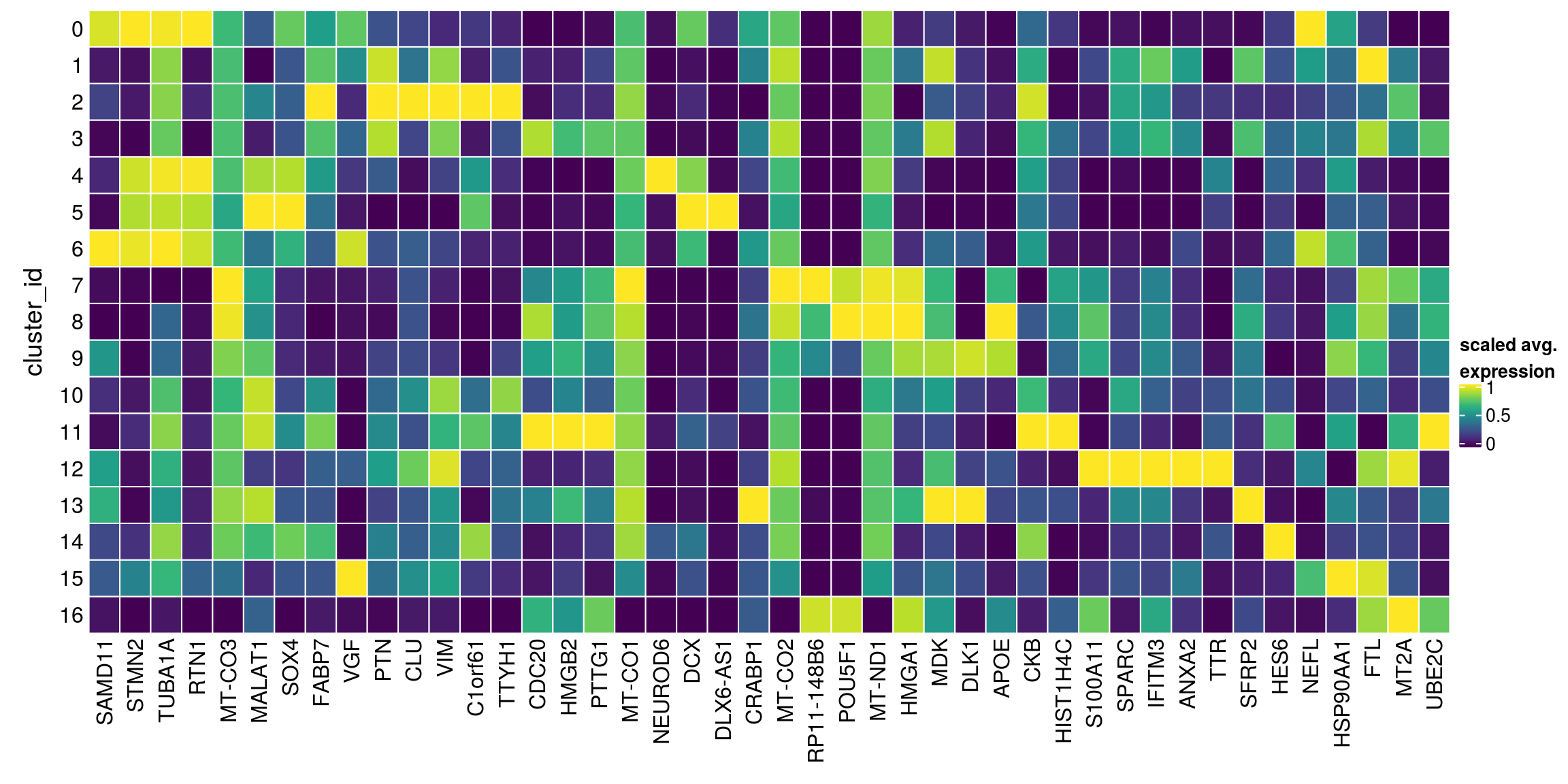
| Version | Author | Date |
|---|---|---|
| 48fb578 | khembach | 2020-09-07 |
We write tables with the top marker genes per cluster.
gs2 <- lapply(scran_markers, function(u) u[u$Top %in% 1:3,])
for (i in seq_along(gs2)) {
  write.table(x = gs2[[i]] %>% as.data.frame %>%
                dplyr::mutate(gene = rownames(gs2[[i]])) %>%
                dplyr::relocate(gene),
              file =  file.path("output",
                                paste0("organoid_integration_cluster", i, "_marker_genes.txt")),
              sep = "\t", quote = FALSE, row.names = FALSE)
}
Heatmap including marker genes of rank 2 and 3.
gs <- lapply(scran_markers, function(u) rownames(u)[u$Top %in% 1:3])
## candidate cluster markers
lapply(gs, function(x) str_split(x, pattern = "\\.", simplify = TRUE)[,2])
$`0`
[1] "SAMD11" "STMN2" "TUBA1A" "RTN1" "MT-CO3" "MALAT1" "NOC2L" "TUBB2A"
[9] "SOX4" "DCX" "MT-CO2" "KLHL17" "CRABP1" "MT-ND4"
$`1`
[1] "SAMD11" "SOX4" "FABP7" "VGF" "PTN" "CLU" "VIM" "TUBA1A"
[9] "MALAT1" "NOC2L" "TUBB2A" "TUBB2B" "NEFL" "STMN2" "CKB" "KLHL17"
[17] "IGFBP2" "BASP1" "PTPRZ1" "LY6H" "METRN" "TTYH1" "MT-CO1"
$`2`
[1] "C1orf61" "FABP7" "PTN" "VIM" "TTYH1" "SOX2" "CKB"
[8] "SAMD11" "IGFBP2" "ATP1B2" "MALAT1"
$`3`
[1] "SAMD11" "CDC20" "HMGB2" "PTTG1" "VIM" "TUBA1A" "MT-CO1"
[8] "NOC2L" "HMGN2" "CENPF" "CKB" "UBE2S" "MALAT1" "KLHL17"
[15] "FABP7" "PTN" "ARL6IP1" "UBE2C"
$`4`
[1] "SOX4" "NEUROD6" "STMN2" "TUBA1A" "NFIB" "RTN1" "NEUROD2"
[8] "MALAT1" "SAMD11" "NSG1" "GPM6A" "DCX" "MT-CO3"
$`5`
[1] "C1orf61" "STMN2" "TUBA1A" "DCX" "DLX6-AS1" "MALAT1"
[7] "SOX4" "TCF4" "DLX5" "SAMD11" "DLX2"
$`6`
[1] "SAMD11" "STMN2" "TUBA1A" "CRABP1" "MT-CO2" "MALAT1" "NOC2L" "STMN1"
[9] "MLLT11" "SCG2" "HES6" "BASP1" "TUBB2B" "CD24" "RTN1" "MT-CO3"
[17] "KLHL17" "GAP43" "VIM" "SEZ6L2"
$`7`
[1] "SAMD11" "MT-CO1" "RP11-148B6" "POU5F1" "NOC2L"
[6] "MT-ND4" "KLHL17" "HMGA1" "TERF1" "MT-CO2"
$`8`
[1] "SAMD11" "MT-ND1" "POU5F1" "NOC2L" "HMGA1"
[6] "PMAIP1" "APOE" "MT-ND2" "KLHL17" "CD24"
[11] "TERF1" "LDHA" "MT-CO3" "RP11-148B6"
$`9`
[1] "HMGA1" "MDK" "DLK1" "APOE" "MT-CO1"
[6] "CD24" "GPC3" "MT-CO3" "RP11-148B6" "SAMD11"
[11] "MALAT1"
$`10`
[1] "SAMD11" "VIM" "MDK" "CKB" "TTYH1" "MALAT1" "NOC2L" "TUBB2B"
[9] "TUBA1A" "KLHL17" "HES4" "SOX2" "TUBA1B" "MT-CO1"
$`11`
[1] "C1orf61" "HMGB2" "HIST1H4C" "TUBA1A" "MALAT1" "FABP7"
[7] "VIM" "CKB" "TOP2A" "CENPF" "CDK1" "TUBA1B"
[13] "MT-CO1"
$`12`
[1] "S100A11" "SPARC" "VIM" "IFITM3" "ANXA2" "MALAT1" "TTR"
[8] "IGFBP5" "PTN" "CLU" "TAGLN" "LGALS1" "MT-CO1" "ID3"
[15] "IGFBP2" "TUBA1A" "TPM1" "MT-CYB"
$`13`
[1] "SFRP2" "MDK" "CRABP1" "MALAT1" "SAMD11" "VIM" "TUBA1A" "MT-CO1"
[9] "NOC2L" "DLK1" "MT-CO3"
$`14`
[1] "C1orf61" "HES6" "SOX4" "TUBA1A" "MALAT1" "HES5" "NFIA"
[8] "SOX11" "VIM" "NHLH1" "IGFBP5" "CKB" "TMSB4X" "MT-CO1"
$`15`
[1] "C1orf61" "NEFL" "STMN2" "VIM" "TUBA1A" "HSP90AA1"
[7] "FTL" "MALAT1" "SOX11" "IGFBP2" "SQSTM1" "VGF"
[13] "DDIT3" "MT-CO1" "SCG2" "TUBB2B" "STMN4" "RPL12"
[19] "FTH1" "SLC3A2" "HSPH1" "RPS27L" "MAP1LC3B"
$`16`
[1] "MT2A" "UBE2C" "RP11-148B6" "POU5F1" "HMGA1"
[6] "MT1G" "UGP2" "CD24" sub <- sce[unique(unlist(gs)), ]
pbs <- aggregateData(sub, assay = "logcounts", by = "cluster_id", fun = "mean")
mat <- t(muscat:::.scale(assay(pbs)))
## remove the Ensembl ID from the gene names
colnames(mat) <- str_split(colnames(mat), pattern = "\\.", simplify = TRUE)[,2]
Heatmap(mat,
name = "scaled avg.\nexpression",
col = viridis(10),
cluster_rows = FALSE,
cluster_columns = FALSE,
row_names_side = "left",
row_title = "cluster_id",
rect_gp = gpar(col = "white"))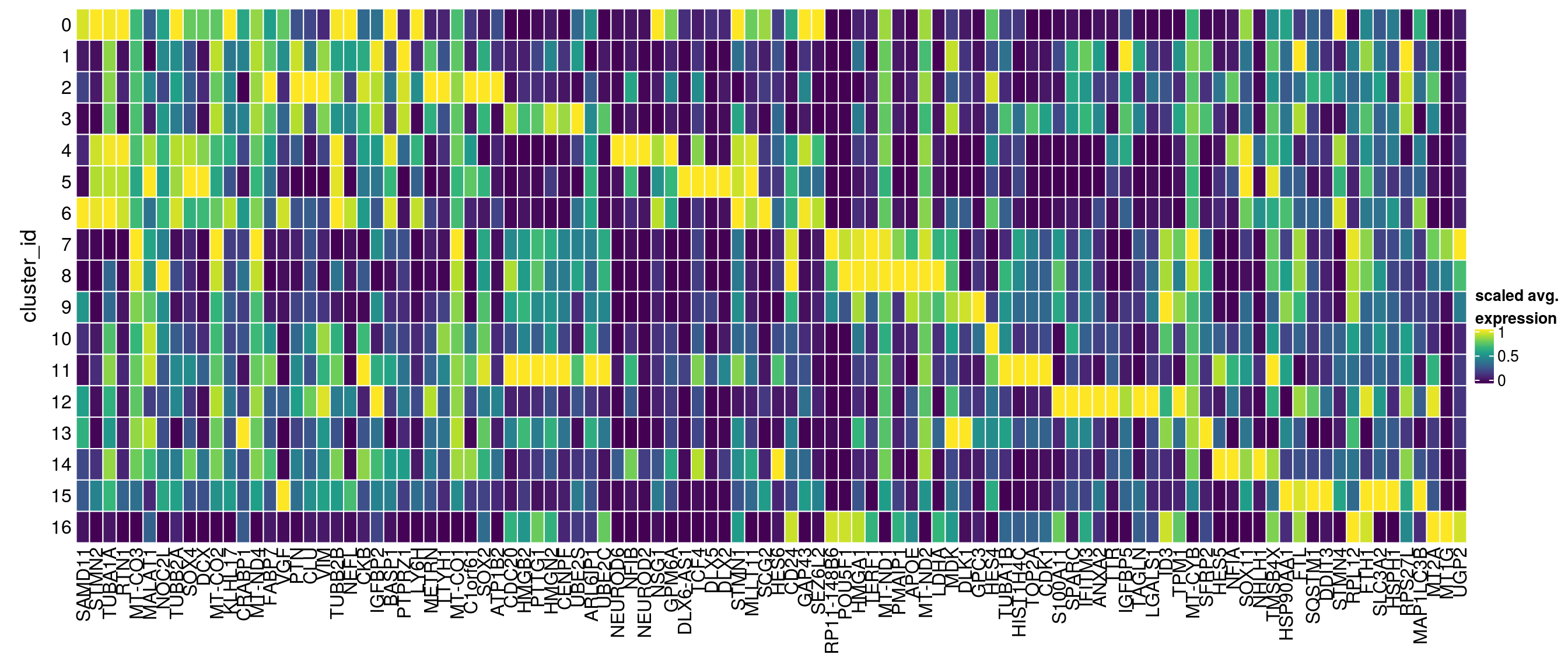
| Version | Author | Date |
|---|---|---|
| 48fb578 | khembach | 2020-09-07 |
sessionInfo()R version 4.0.0 (2020-04-24)
Platform: x86_64-pc-linux-gnu (64-bit)
Running under: Ubuntu 16.04.6 LTS
Matrix products: default
BLAS: /usr/local/R/R-4.0.0/lib/libRblas.so
LAPACK: /usr/local/R/R-4.0.0/lib/libRlapack.so
locale:
[1] LC_CTYPE=en_US.UTF-8 LC_NUMERIC=C
[3] LC_TIME=en_US.UTF-8 LC_COLLATE=en_US.UTF-8
[5] LC_MONETARY=en_US.UTF-8 LC_MESSAGES=en_US.UTF-8
[7] LC_PAPER=en_US.UTF-8 LC_NAME=C
[9] LC_ADDRESS=C LC_TELEPHONE=C
[11] LC_MEASUREMENT=en_US.UTF-8 LC_IDENTIFICATION=C
attached base packages:
[1] parallel stats4 grid stats graphics grDevices utils
[8] datasets methods base
other attached packages:
[1] viridis_0.5.1 viridisLite_0.3.0
[3] stringr_1.4.0 scran_1.16.0
[5] SingleCellExperiment_1.10.1 SummarizedExperiment_1.18.1
[7] DelayedArray_0.14.0 matrixStats_0.56.0
[9] Biobase_2.48.0 GenomicRanges_1.40.0
[11] GenomeInfoDb_1.24.2 IRanges_2.22.2
[13] S4Vectors_0.26.1 BiocGenerics_0.34.0
[15] Seurat_3.1.5 RColorBrewer_1.1-2
[17] muscat_1.2.1 dplyr_1.0.2
[19] ggplot2_3.3.2 cowplot_1.0.0
[21] ComplexHeatmap_2.4.2 workflowr_1.6.2
loaded via a namespace (and not attached):
[1] backports_1.1.9 circlize_0.4.10
[3] blme_1.0-4 igraph_1.2.5
[5] plyr_1.8.6 lazyeval_0.2.2
[7] TMB_1.7.16 splines_4.0.0
[9] BiocParallel_1.22.0 listenv_0.8.0
[11] scater_1.16.2 digest_0.6.25
[13] foreach_1.5.0 htmltools_0.5.0
[15] gdata_2.18.0 lmerTest_3.1-2
[17] magrittr_1.5 memoise_1.1.0
[19] cluster_2.1.0 doParallel_1.0.15
[21] ROCR_1.0-11 limma_3.44.3
[23] globals_0.12.5 annotate_1.66.0
[25] prettyunits_1.1.1 colorspace_1.4-1
[27] rappdirs_0.3.1 ggrepel_0.8.2
[29] blob_1.2.1 xfun_0.15
[31] jsonlite_1.7.0 crayon_1.3.4
[33] RCurl_1.98-1.2 genefilter_1.70.0
[35] lme4_1.1-23 zoo_1.8-8
[37] ape_5.4 survival_3.2-3
[39] iterators_1.0.12 glue_1.4.2
[41] gtable_0.3.0 zlibbioc_1.34.0
[43] XVector_0.28.0 leiden_0.3.3
[45] GetoptLong_1.0.1 BiocSingular_1.4.0
[47] future.apply_1.6.0 shape_1.4.4
[49] scales_1.1.1 DBI_1.1.0
[51] edgeR_3.30.3 Rcpp_1.0.5
[53] xtable_1.8-4 progress_1.2.2
[55] clue_0.3-57 dqrng_0.2.1
[57] reticulate_1.16 bit_1.1-15.2
[59] rsvd_1.0.3 tsne_0.1-3
[61] htmlwidgets_1.5.1 httr_1.4.1
[63] gplots_3.0.4 ellipsis_0.3.1
[65] ica_1.0-2 farver_2.0.3
[67] pkgconfig_2.0.3 XML_3.99-0.4
[69] uwot_0.1.8 locfit_1.5-9.4
[71] labeling_0.3 tidyselect_1.1.0
[73] rlang_0.4.7 reshape2_1.4.4
[75] later_1.1.0.1 AnnotationDbi_1.50.1
[77] munsell_0.5.0 tools_4.0.0
[79] generics_0.0.2 RSQLite_2.2.0
[81] ggridges_0.5.2 evaluate_0.14
[83] yaml_2.2.1 knitr_1.29
[85] bit64_0.9-7 fs_1.4.2
[87] fitdistrplus_1.1-1 caTools_1.18.0
[89] RANN_2.6.1 purrr_0.3.4
[91] pbapply_1.4-2 future_1.17.0
[93] nlme_3.1-148 whisker_0.4
[95] pbkrtest_0.4-8.6 compiler_4.0.0
[97] plotly_4.9.2.1 beeswarm_0.2.3
[99] png_0.1-7 variancePartition_1.18.2
[101] tibble_3.0.3 statmod_1.4.34
[103] geneplotter_1.66.0 stringi_1.4.6
[105] lattice_0.20-41 Matrix_1.2-18
[107] nloptr_1.2.2.2 vctrs_0.3.4
[109] pillar_1.4.6 lifecycle_0.2.0
[111] lmtest_0.9-37 GlobalOptions_0.1.2
[113] RcppAnnoy_0.0.16 BiocNeighbors_1.6.0
[115] data.table_1.12.8 bitops_1.0-6
[117] irlba_2.3.3 patchwork_1.0.1
[119] httpuv_1.5.4 colorRamps_2.3
[121] R6_2.4.1 promises_1.1.1
[123] KernSmooth_2.23-17 gridExtra_2.3
[125] vipor_0.4.5 codetools_0.2-16
[127] boot_1.3-25 MASS_7.3-51.6
[129] gtools_3.8.2 DESeq2_1.28.1
[131] rprojroot_1.3-2 rjson_0.2.20
[133] withr_2.2.0 sctransform_0.2.1
[135] GenomeInfoDbData_1.2.3 hms_0.5.3
[137] tidyr_1.1.0 glmmTMB_1.0.2.1
[139] minqa_1.2.4 rmarkdown_2.3
[141] DelayedMatrixStats_1.10.1 Rtsne_0.15
[143] git2r_0.27.1 numDeriv_2016.8-1.1
[145] ggbeeswarm_0.6.0