Last updated: 2020-08-14
Checks: 7 0
Knit directory: neural_scRNAseq/
This reproducible R Markdown analysis was created with workflowr (version 1.6.2). The Checks tab describes the reproducibility checks that were applied when the results were created. The Past versions tab lists the development history.
Great! Since the R Markdown file has been committed to the Git repository, you know the exact version of the code that produced these results.
Great job! The global environment was empty. Objects defined in the global environment can affect the analysis in your R Markdown file in unknown ways. For reproduciblity it's best to always run the code in an empty environment.
The command set.seed(20200522) was run prior to running the code in the R Markdown file. Setting a seed ensures that any results that rely on randomness, e.g. subsampling or permutations, are reproducible.
Great job! Recording the operating system, R version, and package versions is critical for reproducibility.
Nice! There were no cached chunks for this analysis, so you can be confident that you successfully produced the results during this run.
Great job! Using relative paths to the files within your workflowr project makes it easier to run your code on other machines.
Great! You are using Git for version control. Tracking code development and connecting the code version to the results is critical for reproducibility.
The results in this page were generated with repository version 31bdfcb. See the Past versions tab to see a history of the changes made to the R Markdown and HTML files.
Note that you need to be careful to ensure that all relevant files for the analysis have been committed to Git prior to generating the results (you can use wflow_publish or wflow_git_commit). workflowr only checks the R Markdown file, but you know if there are other scripts or data files that it depends on. Below is the status of the Git repository when the results were generated:
Ignored files:
    Ignored:    .DS_Store
    Ignored:    .Rhistory
    Ignored:    .Rproj.user/
    Ignored:    ._.DS_Store
    Ignored:    ._Rplots.pdf
    Ignored:    .__workflowr.yml
    Ignored:    ._neural_scRNAseq.Rproj
    Ignored:    analysis/.DS_Store
    Ignored:    analysis/.Rhistory
    Ignored:    analysis/._.DS_Store
    Ignored:    analysis/._01-preprocessing.Rmd
    Ignored:    analysis/._01-preprocessing.html
    Ignored:    analysis/._02.1-SampleQC.Rmd
    Ignored:    analysis/._03-filtering.Rmd
    Ignored:    analysis/._04-clustering.Rmd
    Ignored:    analysis/._04-clustering.knit.md
    Ignored:    analysis/._04.1-cell_cycle.Rmd
    Ignored:    analysis/._05-annotation.Rmd
    Ignored:    analysis/._Lam-0-NSC_no_integration.Rmd
    Ignored:    analysis/._Lam-01-NSC_integration.Rmd
    Ignored:    analysis/._Lam-02-NSC_annotation.Rmd
    Ignored:    analysis/._NSC-1-clustering.Rmd
    Ignored:    analysis/._NSC-2-annotation.Rmd
    Ignored:    analysis/.__site.yml
    Ignored:    analysis/._additional_filtering.Rmd
    Ignored:    analysis/._additional_filtering_clustering.Rmd
    Ignored:    analysis/._index.Rmd
    Ignored:    analysis/._organoid-01-clustering.Rmd
    Ignored:    analysis/._organoid-02-integration.Rmd
    Ignored:    analysis/01-preprocessing_cache/
    Ignored:    analysis/02-1-SampleQC_cache/
    Ignored:    analysis/02-quality_control_cache/
    Ignored:    analysis/02.1-SampleQC_cache/
    Ignored:    analysis/03-filtering_cache/
    Ignored:    analysis/04-clustering_cache/
    Ignored:    analysis/04.1-cell_cycle_cache/
    Ignored:    analysis/05-annotation_cache/
    Ignored:    analysis/Lam-01-NSC_integration_cache/
    Ignored:    analysis/Lam-02-NSC_annotation_cache/
    Ignored:    analysis/NSC-1-clustering_cache/
    Ignored:    analysis/NSC-2-annotation_cache/
    Ignored:    analysis/additional_filtering_cache/
    Ignored:    analysis/additional_filtering_clustering_cache/
    Ignored:    analysis/organoid-01-clustering_cache/
    Ignored:    analysis/sample5_QC_cache/
    Ignored:    data/.DS_Store
    Ignored:    data/._.DS_Store
    Ignored:    data/._.smbdeleteAAA17ed8b4b
    Ignored:    data/._Lam_figure2_markers.R
    Ignored:    data/._known_NSC_markers.R
    Ignored:    data/._known_cell_type_markers.R
    Ignored:    data/._metadata.csv
    Ignored:    data/data_sushi/
    Ignored:    data/filtered_feature_matrices/
    Ignored:    output/.DS_Store
    Ignored:    output/._.DS_Store
    Ignored:    output/._NSC_cluster1_marker_genes.txt
    Ignored:    output/Lam-01-clustering.rds
    Ignored:    output/NSC_1_clustering.rds
    Ignored:    output/NSC_cluster1_marker_genes.txt
    Ignored:    output/NSC_cluster2_marker_genes.txt
    Ignored:    output/NSC_cluster3_marker_genes.txt
    Ignored:    output/NSC_cluster4_marker_genes.txt
    Ignored:    output/NSC_cluster5_marker_genes.txt
    Ignored:    output/NSC_cluster6_marker_genes.txt
    Ignored:    output/NSC_cluster7_marker_genes.txt
    Ignored:    output/additional_filtering.rds
    Ignored:    output/figures/
    Ignored:    output/sce_01_preprocessing.rds
    Ignored:    output/sce_02_quality_control.rds
    Ignored:    output/sce_03_filtering.rds
    Ignored:    output/sce_organoid-01-clustering.rds
    Ignored:    output/sce_preprocessing.rds
    Ignored:    output/so_04_1_cell_cycle.rds
    Ignored:    output/so_04_clustering.rds
    Ignored:    output/so_additional_filtering_clustering.rds
    Ignored:    output/so_merged_organoid-02-integration.rds
    Ignored:    output/so_organoid-01-clustering.rds
    Ignored:    output/so_sample_organoid-01-clustering.rds

Untracked files:
    Untracked:  Rplots.pdf
    Untracked:  analysis/Lam-0-NSC_no_integration.Rmd
    Untracked:  analysis/additional_filtering.Rmd
    Untracked:  analysis/additional_filtering_clustering.Rmd
    Untracked:  analysis/organoid-01-integration.Rmd
    Untracked:  analysis/sample5_QC.Rmd
    Untracked:  data/Homo_sapiens.GRCh38.98.sorted.gtf
    Untracked:  data/Kanton_et_al/
    Untracked:  data/Lam_et_al/
    Untracked:  scripts/

Unstaged changes:
    Modified:   analysis/_site.yml
Note that any generated files, e.g. HTML, png, CSS, etc., are not included in this status report because it is ok for generated content to have uncommitted changes.
These are the previous versions of the repository in which changes were made to the R Markdown (analysis/organoid-02-integration.Rmd) and HTML (docs/organoid-02-integration.html) files. If you've configured a remote Git repository (see ?wflow_git_remote), click on the hyperlinks in the table below to view the files as they were in that past version.
| File | Version | Author | Date | Message |
|---|---|---|---|---|
| Rmd | 31bdfcb | khembach | 2020-08-14 | integrate organoid data |
Load packages
library(BiocParallel)
library(ggplot2)
library(dplyr)
library(cowplot)
library(ggplot2)
library(Seurat)
library(SingleCellExperiment)
library(future)
# increase future's maximum allowed size of exported globals
# the default is 2GB
options(future.globals.maxSize = 11000 * 1024 ^ 2)
# change the current plan to access parallelization
plan("multiprocess", workers = 20)Load data & convert to SCE
so_nsc <- readRDS(file.path("output", "so_04_clustering.rds"))
DefaultAssay(so_nsc) <- "RNA"
so_org <- readRDS(file.path("output", "so_organoid-01-clustering.rds"))
DefaultAssay(so_org) <- "RNA"Clustering without integration
We merge the normalized Seurat objects of our NSCs and neural cultures and the human organoid data from Kanton et al. 2019. Then we run PCA, tSNE, UMAP and clustering. We want to know if there are big differences between the two datasets that make an integration necessary.
so <- merge(so_nsc, y = so_org, add.cell.ids = c("NSC", "organoid"),
            project = "neural_cultures", merge.data = TRUE)
## variable with sample ID from our data and cell line from organoids
so$merged_sample <- ifelse(!is.na(so$Line), so$Line, so$sample_id)
## variable with group ID from our data and Stage from organoids
so$merged_group <-  ifelse(!is.na(so$group_id), so$group_id, so$Stage)
## variable with number of UMIs and fraction of MT UMIs
so$merged_nUMIs <- ifelse(!is.na(so$sum), so$sum, so$nUMI)
so$merged_fractionMt <- ifelse(!is.na(so$subsets_Mt_fraction),
                              so$subsets_Mt_fraction, so$PercentMito)
so$merged_nGenes <- ifelse(!is.na(so$detected), so$detected, so$nGene)
so <- FindVariableFeatures(so, nfeatures = 2000,
selection.method = "vst", verbose = FALSE)
so <- ScaleData(so, verbose = FALSE,
vars.to.regress = c("merged_nUMIs", "merged_fractionMt"))so <- RunPCA(so, npcs = 30, verbose = FALSE)
so <- RunTSNE(so, reduction = "pca", dims = seq_len(20),
seed.use = 1, do.fast = TRUE, verbose = FALSE)
so <- RunUMAP(so, reduction = "pca", dims = seq_len(20),
seed.use = 1, verbose = FALSE)Warning: The default method for RunUMAP has changed from calling Python UMAP via reticulate to the R-native UWOT using the cosine metric
To use Python UMAP via reticulate, set umap.method to 'umap-learn' and metric to 'correlation'
This message will be shown once per sessionDimPlot(so, reduction = "pca", group.by = "merged_sample")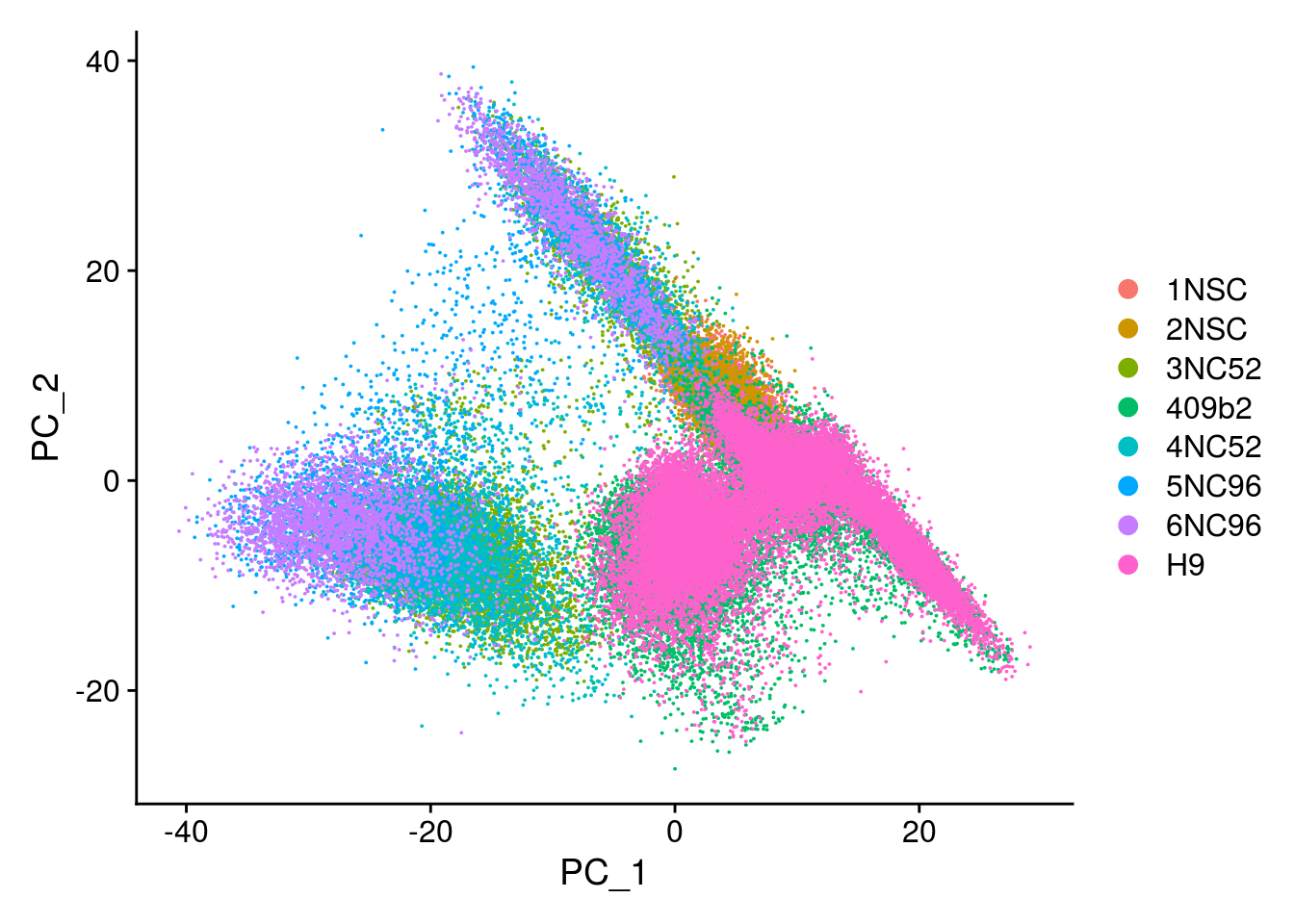
so <- FindNeighbors(so, reduction = "pca", dims = seq_len(20), verbose = FALSE)
so <- FindClusters(so, resolution = 0.4, random.seed = 1, verbose = FALSE)
Dimension reduction plots
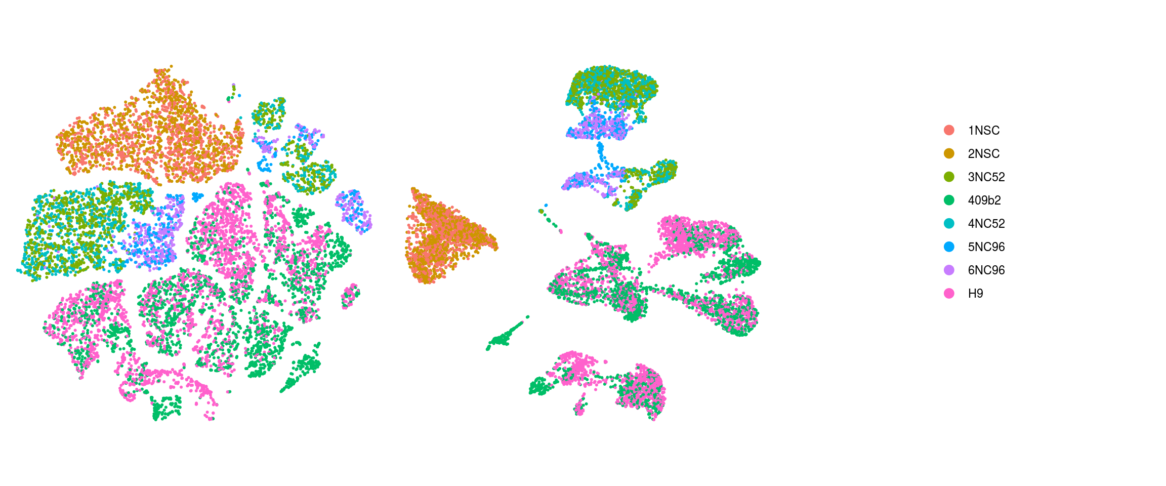
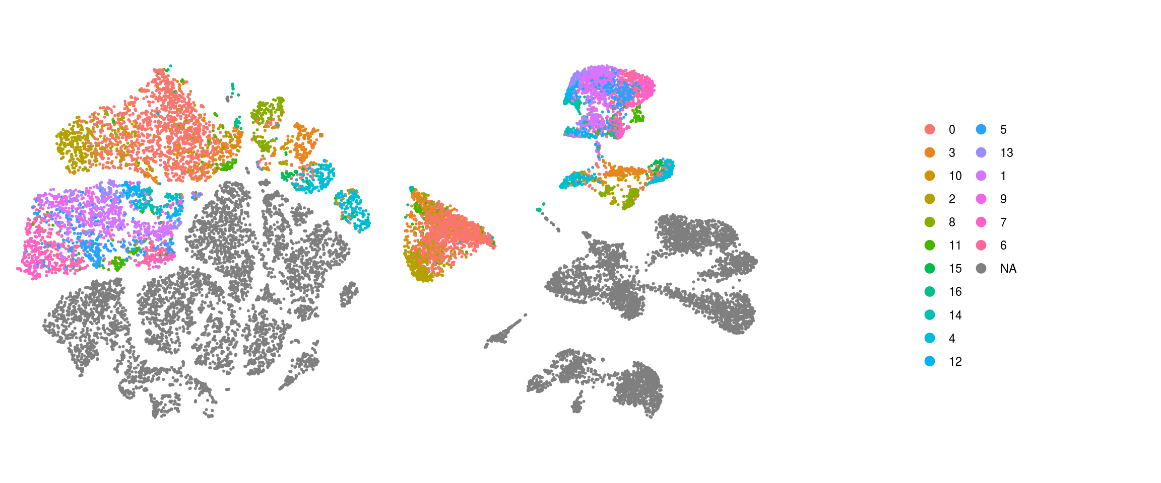
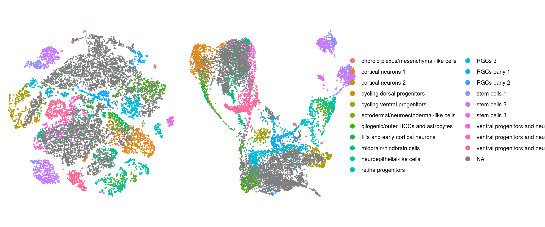
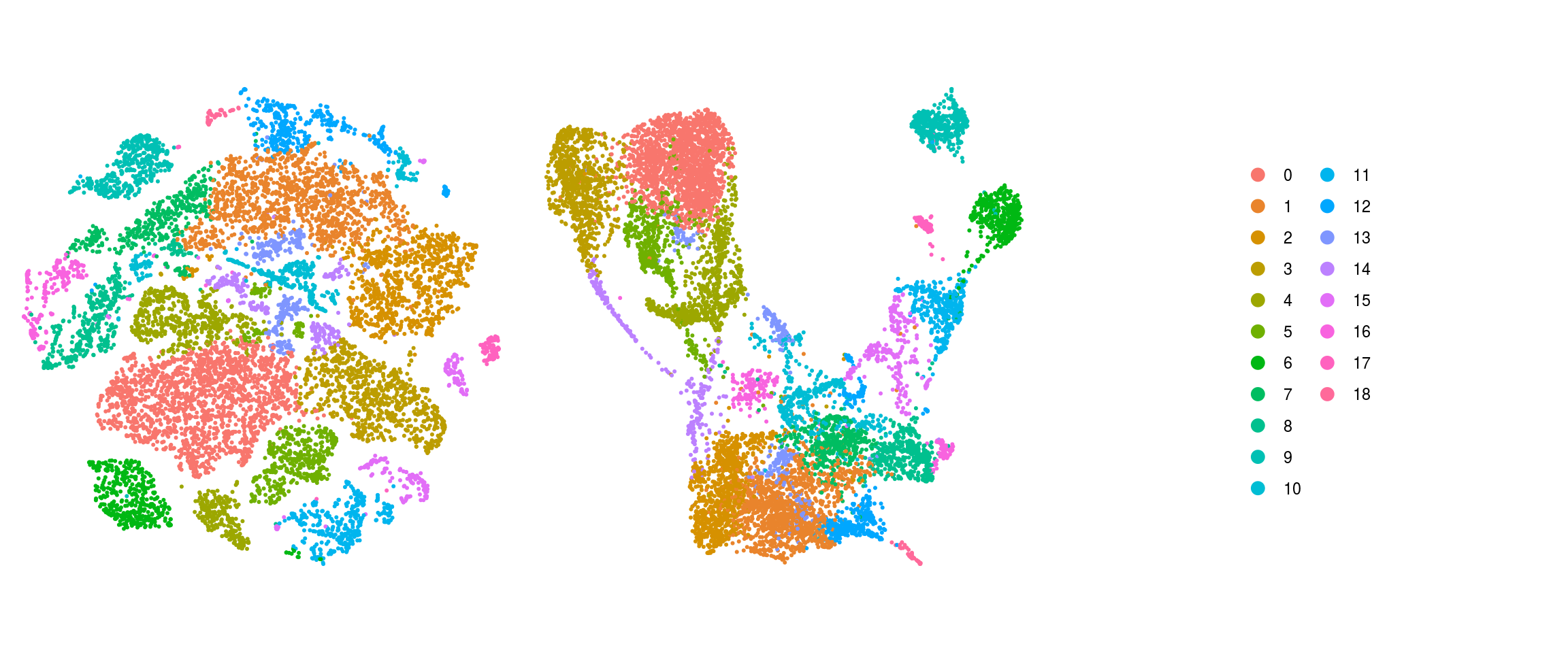
We plot the dimension reduction (DR) and color by same/cell line, group/Stage, organoid cluster labels, cluster ID
# set cluster IDs to resolution 0.4 clustering
so <- SetIdent(so, value = "integrated_snn_res.0.4")
so@meta.data$cluster_id <- Idents(so)

cs <- sample(colnames(so), 10e3)
.plot_dr <- function(so, dr, id)
    DimPlot(so, cells = cs, group.by = id, reduction = dr, pt.size = 0.4) +
        guides(col = guide_legend(nrow = 11,
            override.aes = list(size = 3, alpha = 1))) +
        theme_void() + theme(aspect.ratio = 1)
ids <- c("merged_sample", "merged_group","cl_FullLineage", "ident")
for (id in ids) {
    cat("### ", id, "\n")
    p1 <- .plot_dr(so, "tsne", id)
    lgd <- get_legend(p1)
    p1 <- p1 + theme(legend.position = "none")
    p2 <- .plot_dr(so, "umap", id) + theme(legend.position = "none")
    ps <- plot_grid(plotlist = list(p1, p2), nrow = 1)
    p <- plot_grid(ps, lgd, nrow = 1, rel_widths = c(1, 0.5))
    print(p)
    cat("\n\n")
}
merged_sample
merged_group
cl_FullLineage
ident
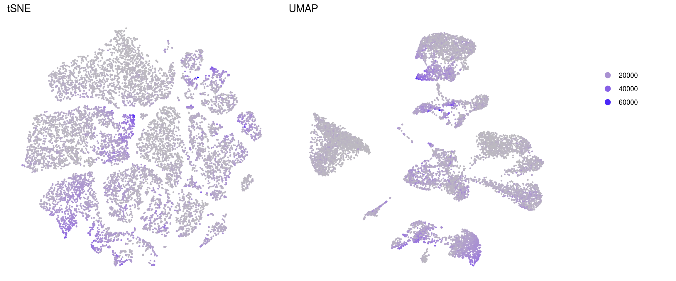
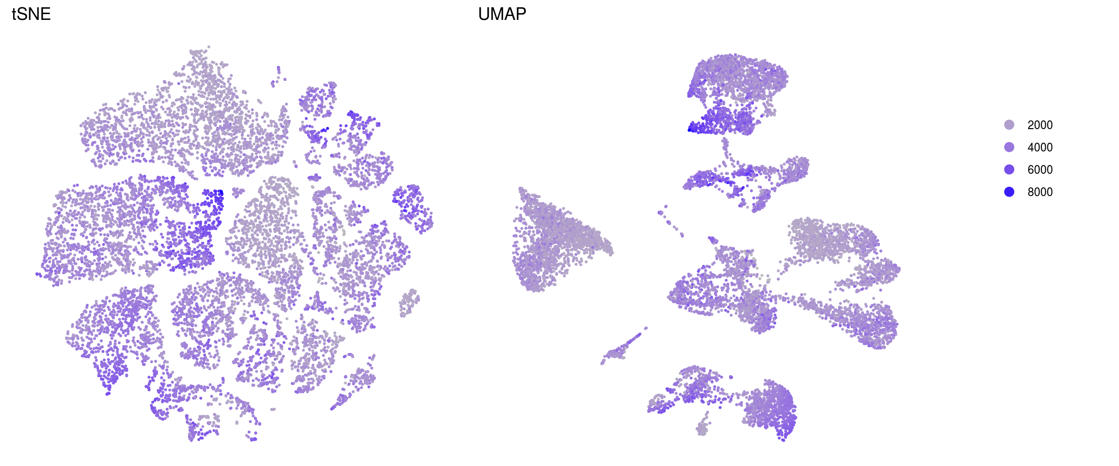
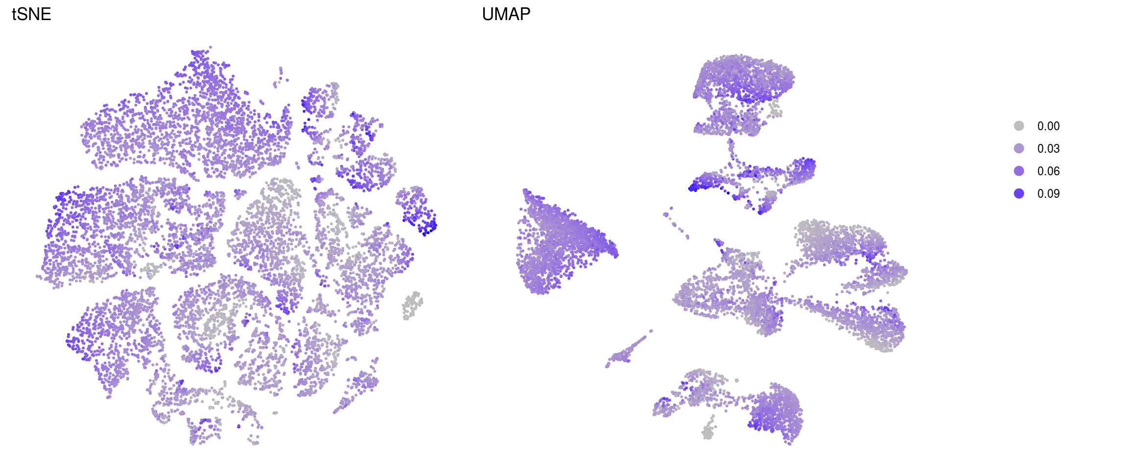
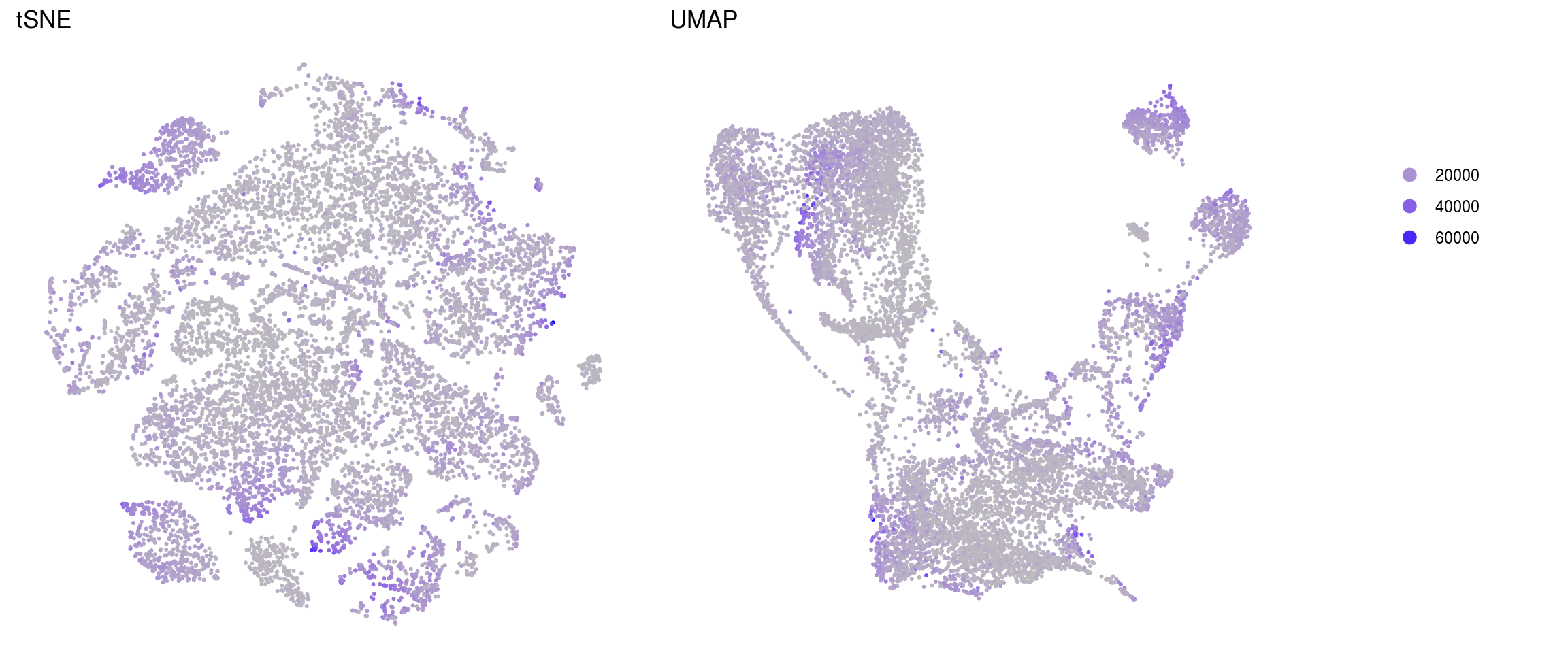
QC on DR plots
.plot_features <- function(so, dr, id) {
    FeaturePlot(so, cells = cs, features = id, reduction = dr, pt.size = 0.4,
                cols = c("grey", "blue")) +
        guides(col = guide_legend(nrow = 11,
            override.aes = list(size = 3, alpha = 1))) +
        theme_void() + theme(aspect.ratio = 1)
}
ids <- c("merged_nUMIs", "merged_nGenes", "merged_fractionMt")
for (id in ids) {
    cat("### ", id, "\n")
    p1 <- .plot_features(so, "tsne", id)
    lgd <- get_legend(p1)
    p1 <- p1 + theme(legend.position = "none") + ggtitle("tSNE")
    p2 <- .plot_features(so, "umap", id) + theme(legend.position = "none") +
      ggtitle("UMAP")
    ps <- plot_grid(plotlist = list(p1, p2), nrow = 1)
    p <- plot_grid(ps, lgd, nrow = 1, rel_widths = c(1, 0.2))
    print(p)
    cat("\n\n")
}
merged_nUMIs
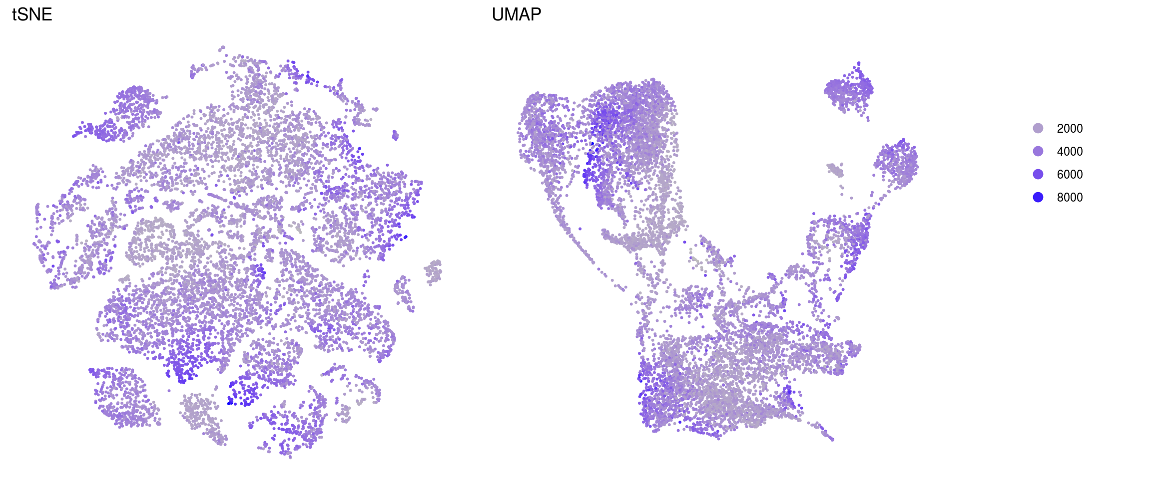
merged_nGenes
merged_fractionMt
Save Seurat object to RDS
saveRDS(so, file.path("output", "so_merged_organoid-02-integration.rds"))Integration
We integrate the two datasets because they are completely separated in the DR plots (see above).
## make sure column names match between datasets:
## we will use sample_id, group_id, nUMI, fractionMt, nGene
so_nsc$nUMI <- so_nsc$sum
so_nsc$fractionMt <- so_nsc$subsets_Mt_fraction
so_nsc$nGene <- so_nsc$detected
so_nsc$sum <- NULL
so_nsc$subsets_Mt_fraction <- NULL
so_nsc$detected <- NULL
so_org$sample_id <- so_org$Line
so_org$group_id <- so_org$Stage
so_org$fractionMt <- so_org$PercentMito
so_org$Line <- NULL
so_org$Stage <- NULL
so_org$PercentMito <- NULL

# split our cells by sample
cells_by_sample <- split(colnames(so_nsc), so_nsc$sample_id)
so_nsc <- lapply(cells_by_sample, function(i) subset(so_nsc, cells = i))
# split organoid cells by cell Line
cells_by_sample <- split(colnames(so_org), so_org$sample_id)
so_org <- lapply(cells_by_sample, function(i) subset(so_org, cells = i))
## we combine the two lists
so <- c(so_nsc, so_org)

## Identify the top 2000 genes with high cell-to-cell variation
so <- lapply(so, FindVariableFeatures, nfeatures = 2000,
    selection.method = "vst", verbose = FALSE)
## find anchors & integrate
as <- FindIntegrationAnchors(so, verbose = FALSE)
so <- IntegrateData(anchorset = as, dims = seq_len(30), verbose = FALSE)DefaultAssay(so) <- "integrated"
## We scale the data
so <- ScaleData(so, verbose = FALSE,
vars.to.regress = c("nUMI", "fractionMt"))so <- RunPCA(so, npcs = 30, verbose = FALSE)
so <- RunTSNE(so, reduction = "pca", dims = seq_len(20),
seed.use = 1, do.fast = TRUE, verbose = FALSE)
so <- RunUMAP(so, reduction = "pca", dims = seq_len(20),
seed.use = 1, verbose = FALSE)
## PCA plot
DimPlot(so, reduction = "pca", group.by = "sample_id")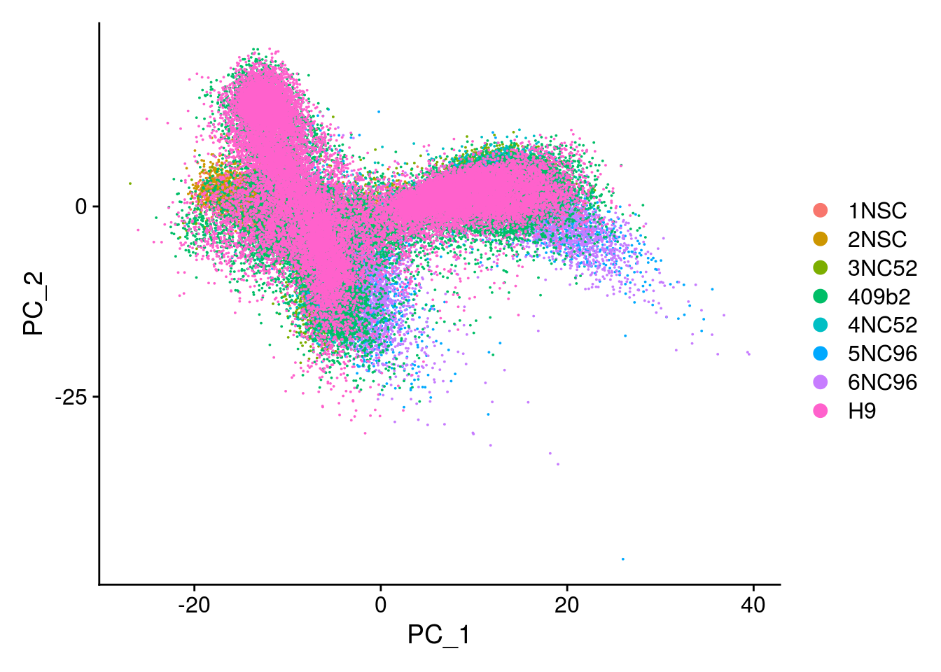
# elbow plot with the ranking of PCs based on the % of variance explained
ElbowPlot(so, ndims = 30)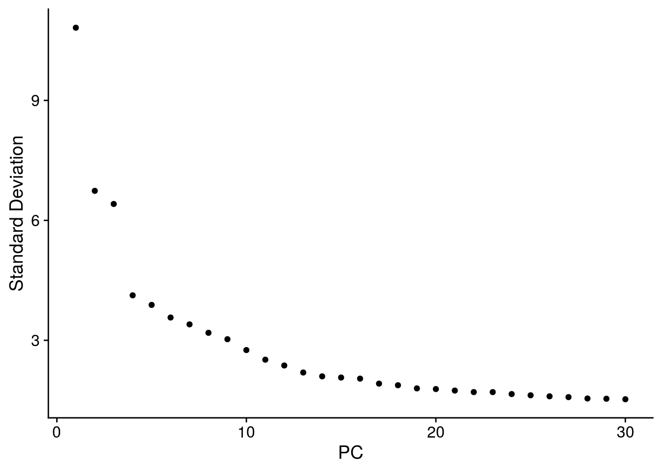
so <- FindNeighbors(so, reduction = "pca", dims = seq_len(20), verbose = FALSE)
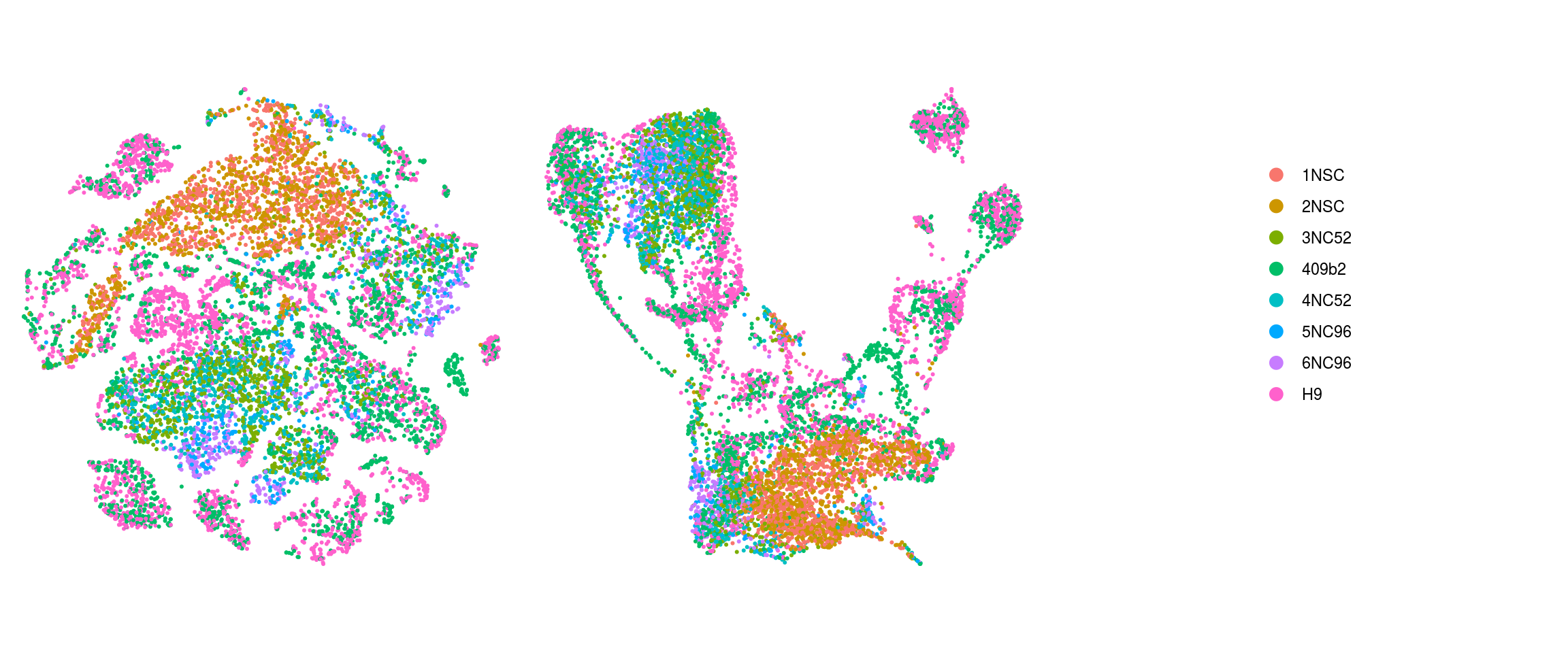
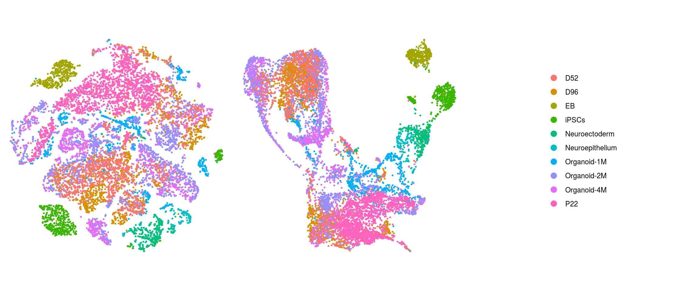
so <- FindClusters(so, resolution = 0.4, random.seed = 1, verbose = FALSE)Dimension reduction plots
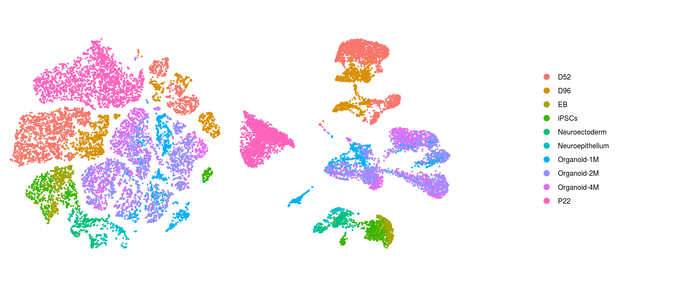
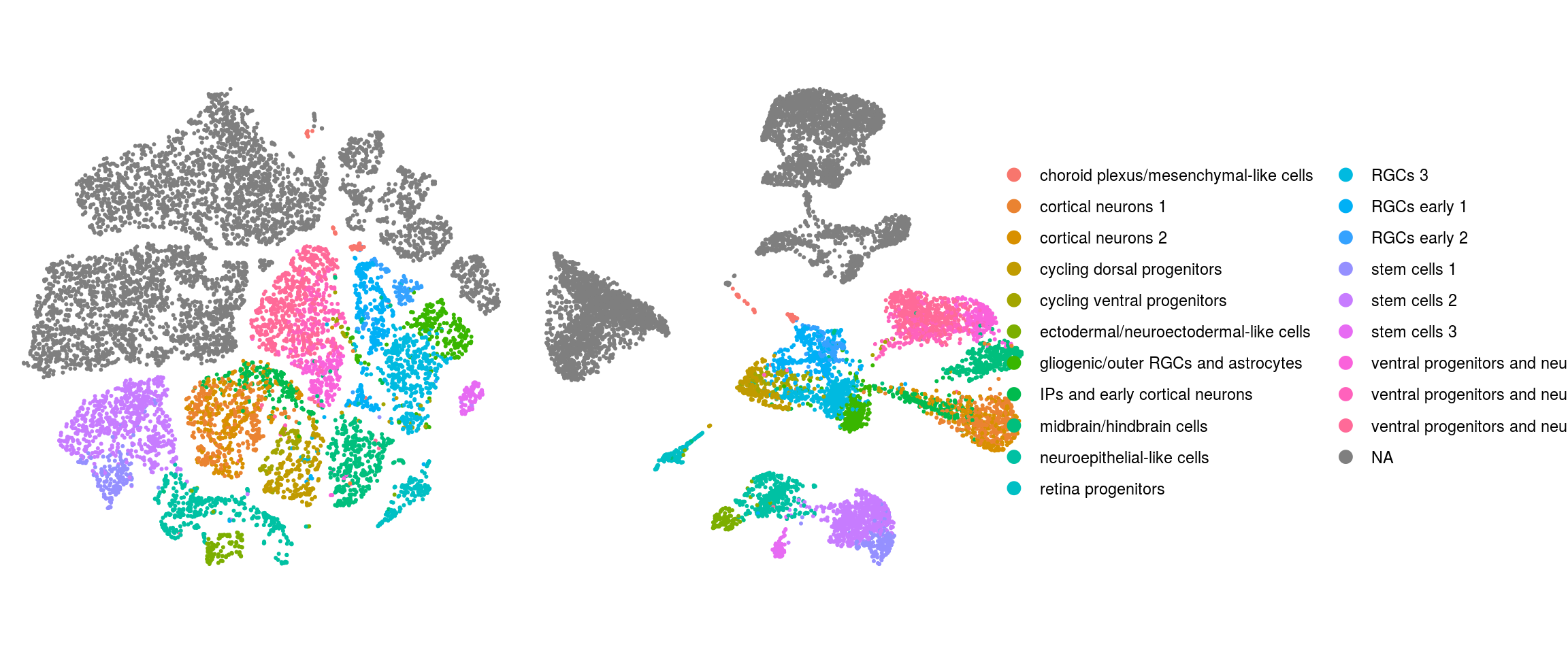
We plot the dimension reduction (DR) and color by same/cell line, group/Stage, organoid cluster labels, cluster ID
# set cluster IDs to resolution 0.4 clustering
so <- SetIdent(so, value = "integrated_snn_res.0.4")
so@meta.data$cluster_id <- Idents(so)

cs <- sample(colnames(so), 10e3)
.plot_dr <- function(so, dr, id)
    DimPlot(so, cells = cs, group.by = id, reduction = dr, pt.size = 0.4) +
        guides(col = guide_legend(nrow = 11,
            override.aes = list(size = 3, alpha = 1))) +
        theme_void() + theme(aspect.ratio = 1)
ids <- c("sample_id", "group_id", "cl_FullLineage", "ident")
for (id in ids) {
    cat("### ", id, "\n")
    p1 <- .plot_dr(so, "tsne", id)
    lgd <- get_legend(p1)
    p1 <- p1 + theme(legend.position = "none")
    p2 <- .plot_dr(so, "umap", id) + theme(legend.position = "none")
    ps <- plot_grid(plotlist = list(p1, p2), nrow = 1)
    p <- plot_grid(ps, lgd, nrow = 1, rel_widths = c(1, 0.5))
    print(p)
    cat("\n\n")
}
sample_id
group_id
cl_FullLineage
ident
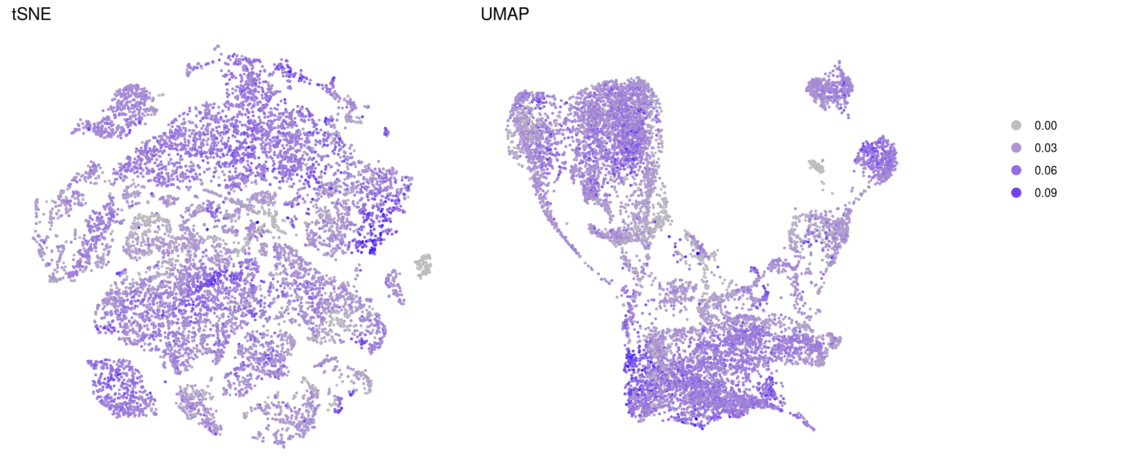
QC on DR plots
.plot_features <- function(so, dr, id) {
    FeaturePlot(so, cells = cs, features = id, reduction = dr, pt.size = 0.4,
                cols = c("grey", "blue")) +
        guides(col = guide_legend(nrow = 11,
            override.aes = list(size = 3, alpha = 1))) +
        theme_void() + theme(aspect.ratio = 1)
}
ids <- c("nUMI", "nGene", "fractionMt")
for (id in ids) {
    cat("### ", id, "\n")
    p1 <- .plot_features(so, "tsne", id)
    lgd <- get_legend(p1)
    p1 <- p1 + theme(legend.position = "none") + ggtitle("tSNE")
    p2 <- .plot_features(so, "umap", id) + theme(legend.position = "none") +
      ggtitle("UMAP")
    ps <- plot_grid(plotlist = list(p1, p2), nrow = 1)
    p <- plot_grid(ps, lgd, nrow = 1, rel_widths = c(1, 0.2))
    print(p)
    cat("\n\n")
}
nUMI
nGene
fractionMt
Save Seurat object to RDS
saveRDS(so, file.path("output", "so_integrated_organoid-02-integration.rds"))
sessionInfo()R version 4.0.0 (2020-04-24)
Platform: x86_64-pc-linux-gnu (64-bit)
Running under: Ubuntu 16.04.6 LTS
Matrix products: default
BLAS: /usr/local/R/R-4.0.0/lib/libRblas.so
LAPACK: /usr/local/R/R-4.0.0/lib/libRlapack.so
locale:
[1] LC_CTYPE=en_US.UTF-8 LC_NUMERIC=C
[3] LC_TIME=en_US.UTF-8 LC_COLLATE=en_US.UTF-8
[5] LC_MONETARY=en_US.UTF-8 LC_MESSAGES=en_US.UTF-8
[7] LC_PAPER=en_US.UTF-8 LC_NAME=C
[9] LC_ADDRESS=C LC_TELEPHONE=C
[11] LC_MEASUREMENT=en_US.UTF-8 LC_IDENTIFICATION=C
attached base packages:
[1] parallel stats4 stats graphics grDevices utils datasets
[8] methods base
other attached packages:
[1] future_1.17.0 SingleCellExperiment_1.10.1
[3] SummarizedExperiment_1.18.1 DelayedArray_0.14.0
[5] matrixStats_0.56.0 Biobase_2.48.0
[7] GenomicRanges_1.40.0 GenomeInfoDb_1.24.2
[9] IRanges_2.22.2 S4Vectors_0.26.1
[11] BiocGenerics_0.34.0 Seurat_3.1.5
[13] cowplot_1.0.0 dplyr_1.0.0
[15] ggplot2_3.3.2 BiocParallel_1.22.0
[17] workflowr_1.6.2
loaded via a namespace (and not attached):
[1] nlme_3.1-148 tsne_0.1-3 bitops_1.0-6
[4] fs_1.4.2 RcppAnnoy_0.0.16 RColorBrewer_1.1-2
[7] httr_1.4.1 rprojroot_1.3-2 sctransform_0.2.1
[10] tools_4.0.0 backports_1.1.8 R6_2.4.1
[13] irlba_2.3.3 KernSmooth_2.23-17 uwot_0.1.8
[16] lazyeval_0.2.2 colorspace_1.4-1 withr_2.2.0
[19] tidyselect_1.1.0 gridExtra_2.3 compiler_4.0.0
[22] git2r_0.27.1 plotly_4.9.2.1 labeling_0.3
[25] scales_1.1.1 lmtest_0.9-37 ggridges_0.5.2
[28] pbapply_1.4-2 rappdirs_0.3.1 stringr_1.4.0
[31] digest_0.6.25 rmarkdown_2.3 XVector_0.28.0
[34] pkgconfig_2.0.3 htmltools_0.5.0 htmlwidgets_1.5.1
[37] rlang_0.4.6 farver_2.0.3 generics_0.0.2
[40] zoo_1.8-8 jsonlite_1.7.0 ica_1.0-2
[43] RCurl_1.98-1.2 magrittr_1.5 GenomeInfoDbData_1.2.3
[46] patchwork_1.0.1 Matrix_1.2-18 Rcpp_1.0.4.6
[49] munsell_0.5.0 ape_5.4 reticulate_1.16
[52] lifecycle_0.2.0 stringi_1.4.6 whisker_0.4
[55] yaml_2.2.1 zlibbioc_1.34.0 MASS_7.3-51.6
[58] Rtsne_0.15 plyr_1.8.6 grid_4.0.0
[61] listenv_0.8.0 promises_1.1.1 ggrepel_0.8.2
[64] crayon_1.3.4 lattice_0.20-41 splines_4.0.0
[67] knitr_1.29 pillar_1.4.4 igraph_1.2.5
[70] future.apply_1.6.0 reshape2_1.4.4 codetools_0.2-16
[73] leiden_0.3.3 glue_1.4.1 evaluate_0.14
[76] data.table_1.12.8 vctrs_0.3.1 png_0.1-7
[79] httpuv_1.5.4 gtable_0.3.0 RANN_2.6.1
[82] purrr_0.3.4 tidyr_1.1.0 xfun_0.15
[85] rsvd_1.0.3 RSpectra_0.16-0 later_1.1.0.1
[88] survival_3.2-3 viridisLite_0.3.0 tibble_3.0.1
[91] cluster_2.1.0 globals_0.12.5 fitdistrplus_1.1-1
[94] ellipsis_0.3.1 ROCR_1.0-11