Organoid integration
Katharina Hembach
8/10/2020
Last updated: 2020-08-18
Checks: 7 0
Knit directory: neural_scRNAseq/
This reproducible R Markdown analysis was created with workflowr (version 1.6.2). The Checks tab describes the reproducibility checks that were applied when the results were created. The Past versions tab lists the development history.
Great! Since the R Markdown file has been committed to the Git repository, you know the exact version of the code that produced these results.
Great job! The global environment was empty. Objects defined in the global environment can affect the analysis in your R Markdown file in unknown ways. For reproduciblity it's best to always run the code in an empty environment.
The command set.seed(20200522) was run prior to running the code in the R Markdown file. Setting a seed ensures that any results that rely on randomness, e.g. subsampling or permutations, are reproducible.
Great job! Recording the operating system, R version, and package versions is critical for reproducibility.
Nice! There were no cached chunks for this analysis, so you can be confident that you successfully produced the results during this run.
Great job! Using relative paths to the files within your workflowr project makes it easier to run your code on other machines.
Great! You are using Git for version control. Tracking code development and connecting the code version to the results is critical for reproducibility.
The results in this page were generated with repository version b960356. See the Past versions tab to see a history of the changes made to the R Markdown and HTML files.
Note that you need to be careful to ensure that all relevant files for the analysis have been committed to Git prior to generating the results (you can use wflow_publish or wflow_git_commit). workflowr only checks the R Markdown file, but you know if there are other scripts or data files that it depends on. Below is the status of the Git repository when the results were generated:
Ignored files:
    Ignored:    .DS_Store
    Ignored:    .Rhistory
    Ignored:    .Rproj.user/
    Ignored:    ._.DS_Store
    Ignored:    ._Rplots.pdf
    Ignored:    .__workflowr.yml
    Ignored:    ._neural_scRNAseq.Rproj
    Ignored:    analysis/.DS_Store
    Ignored:    analysis/.Rhistory
    Ignored:    analysis/._.DS_Store
    Ignored:    analysis/._01-preprocessing.Rmd
    Ignored:    analysis/._01-preprocessing.html
    Ignored:    analysis/._02.1-SampleQC.Rmd
    Ignored:    analysis/._03-filtering.Rmd
    Ignored:    analysis/._04-clustering.Rmd
    Ignored:    analysis/._04-clustering.knit.md
    Ignored:    analysis/._04.1-cell_cycle.Rmd
    Ignored:    analysis/._05-annotation.Rmd
    Ignored:    analysis/._Lam-0-NSC_no_integration.Rmd
    Ignored:    analysis/._Lam-01-NSC_integration.Rmd
    Ignored:    analysis/._Lam-02-NSC_annotation.Rmd
    Ignored:    analysis/._NSC-1-clustering.Rmd
    Ignored:    analysis/._NSC-2-annotation.Rmd
    Ignored:    analysis/.__site.yml
    Ignored:    analysis/._additional_filtering.Rmd
    Ignored:    analysis/._additional_filtering_clustering.Rmd
    Ignored:    analysis/._index.Rmd
    Ignored:    analysis/._organoid-01-clustering.Rmd
    Ignored:    analysis/._organoid-02-integration.Rmd
    Ignored:    analysis/01-preprocessing_cache/
    Ignored:    analysis/02-1-SampleQC_cache/
    Ignored:    analysis/02-quality_control_cache/
    Ignored:    analysis/02.1-SampleQC_cache/
    Ignored:    analysis/03-filtering_cache/
    Ignored:    analysis/04-clustering_cache/
    Ignored:    analysis/04.1-cell_cycle_cache/
    Ignored:    analysis/05-annotation_cache/
    Ignored:    analysis/Lam-01-NSC_integration_cache/
    Ignored:    analysis/Lam-02-NSC_annotation_cache/
    Ignored:    analysis/NSC-1-clustering_cache/
    Ignored:    analysis/NSC-2-annotation_cache/
    Ignored:    analysis/additional_filtering_cache/
    Ignored:    analysis/additional_filtering_clustering_cache/
    Ignored:    analysis/organoid-02-integration_cache/
    Ignored:    analysis/sample5_QC_cache/
    Ignored:    data/.DS_Store
    Ignored:    data/._.DS_Store
    Ignored:    data/._.smbdeleteAAA17ed8b4b
    Ignored:    data/._Lam_figure2_markers.R
    Ignored:    data/._known_NSC_markers.R
    Ignored:    data/._known_cell_type_markers.R
    Ignored:    data/._metadata.csv
    Ignored:    data/data_sushi/
    Ignored:    data/filtered_feature_matrices/
    Ignored:    output/.DS_Store
    Ignored:    output/._.DS_Store
    Ignored:    output/._NSC_cluster1_marker_genes.txt
    Ignored:    output/Lam-01-clustering.rds
    Ignored:    output/NSC_1_clustering.rds
    Ignored:    output/NSC_cluster1_marker_genes.txt
    Ignored:    output/NSC_cluster2_marker_genes.txt
    Ignored:    output/NSC_cluster3_marker_genes.txt
    Ignored:    output/NSC_cluster4_marker_genes.txt
    Ignored:    output/NSC_cluster5_marker_genes.txt
    Ignored:    output/NSC_cluster6_marker_genes.txt
    Ignored:    output/NSC_cluster7_marker_genes.txt
    Ignored:    output/additional_filtering.rds
    Ignored:    output/figures/
    Ignored:    output/sce_01_preprocessing.rds
    Ignored:    output/sce_02_quality_control.rds
    Ignored:    output/sce_03_filtering.rds
    Ignored:    output/sce_organoid-01-clustering.rds
    Ignored:    output/sce_preprocessing.rds
    Ignored:    output/so_04_1_cell_cycle.rds
    Ignored:    output/so_04_clustering.rds
    Ignored:    output/so_additional_filtering_clustering.rds
    Ignored:    output/so_integrated_organoid-02-integration.rds
    Ignored:    output/so_merged_organoid-02-integration.rds
    Ignored:    output/so_organoid-01-clustering.rds
    Ignored:    output/so_sample_organoid-01-clustering.rds

Untracked files:
    Untracked:  Rplots.pdf
    Untracked:  analysis/Lam-0-NSC_no_integration.Rmd
    Untracked:  analysis/additional_filtering.Rmd
    Untracked:  analysis/additional_filtering_clustering.Rmd
    Untracked:  analysis/sample5_QC.Rmd
    Untracked:  data/Homo_sapiens.GRCh38.98.sorted.gtf
    Untracked:  data/Kanton_et_al/
    Untracked:  data/Lam_et_al/
    Untracked:  scripts/

Unstaged changes:
    Modified:   analysis/_site.yml
Note that any generated files, e.g. HTML, png, CSS, etc., are not included in this status report because it is ok for generated content to have uncommitted changes.
These are the previous versions of the repository in which changes were made to the R Markdown (analysis/organoid-01-clustering.Rmd) and HTML (docs/organoid-01-clustering.html) files. If you've configured a remote Git repository (see ?wflow_git_remote), click on the hyperlinks in the table below to view the files as they were in that past version.
| File | Version | Author | Date | Message |
|---|---|---|---|---|
| html | 6405fad | khembach | 2020-08-14 | Build site. |
| Rmd | 638915f | khembach | 2020-08-14 | organoid clustering |
| html | 5b37055 | khembach | 2020-08-12 | Build site. |
| Rmd | ec375b2 | khembach | 2020-08-12 | Cluster organoid data fromn Kanton et al. 2019 |
Load packages
library(DropletUtils)
library(scDblFinder)
library(BiocParallel)
library(ggplot2)
library(scater)
library(dplyr)
library(cowplot)
library(ggplot2)
library(Seurat)
library(SingleCellExperiment)
library(stringr)
library(Seurat)
library(rtracklayer)
library(future)
library(data.table)
# increase future's maximum allowed size of exported globals to 5GB
# the default is 2GB
options(future.globals.maxSize = 5000 * 1024 ^ 2)
# change the current plan to access parallelization
plan("multiprocess", workers = 20)Importing CellRanger output and metadata
fs <- file.path("data", "Kanton_et_al", "files")
sce <- read10xCounts(samples = fs, sample.names = "organoids")

# rename colnames and dimnames
names(rowData(sce)) <- c("ensembl_id", "symbol", "type")
names(colData(sce)) <- c("sample_id", "barcode")

# load metadata
meta <- read.csv(file.path("data", "Kanton_et_al", "metadata.csv"))
colData(sce) <- cbind(colData(sce), meta[, colnames(meta != "Barcode")])

sce$sample_id <- factor(sce$sample_id)
dimnames(sce) <- list(with(rowData(sce), paste(ensembl_id, symbol, sep = ".")),
                      with(colData(sce), paste(barcode, Sample, sep = ".")))
Overview of the data
table(colData(sce)$Line)
  409b2      H9   Hoik1   Kucg2 Sc102a1   Sojd3   Wibj2
  24983   25543    3583    4704   10408    4144   17211
table(colData(sce)$Stage)
             EB           iPSCs   Neuroectoderm Neuroepithelium     Organoid-1M
           3300            4300            2757            1363            5070
    Organoid-2M     Organoid-4M
          62306           11480
table(colData(sce)$Sample)
      h409B2_120d_org1       h409B2_128d_org1        h409B2_60d_org1
                  3179                   3915                   6354
       h409B2_67d_org1              h409B2_EB           h409B2_iPSCs
                  4992                    855                   1943
  h409B2_neuroectoderm h409B2_neuroepithelium         h409B2_Org_32d
                   886                    443                   2416
          H9_128d_org1            H9_60d_org1            H9_67d_org1
                  4386                   5899                   5011
                 H9_EB               H9_iPSCs       H9_neuroectoderm
                  2445                   2357                   1871
    H9_neuroepithelium             H9_Org_32d          hoik_HipSci_1
                   920                   2654                   1168
         hoik_HipSci_2          hoik_HipSci_3          kucg_HipSci_1
                  1533                    882                   1456
         kucg_HipSci_2          kucg_HipSci_3       SC102A1_65d_org1
                  1322                   1926                   5231
      SC102A1_65d_org2          sojd_HipSci_1          sojd_HipSci_2
                  5177                   1247                   1122
         sojd_HipSci_3          wibj_64d_org1          wibj_64d_org2
                  1775                   5823                   6272
         wibj_HipSci_1          wibj_HipSci_2          wibj_HipSci_3
                  1774                   1516                   1826
table(colData(sce)$PredCellType)
     Astrocyte   Astrocyte/RG        Choroid     Choroid/RG             EN
           651              4           1725              1          27146
       EN/Glyc          EN/IN    Endothelial           Glyc        Glyc/IN
            11              7              5          15292              2
Glyc/Microglia     Glyc/Mural        Glyc/RG             IN         IN/IPC
             1              1              4          14482              1
  IN/Microglia            IPC         IPC/RG      Microglia          Mural
             1          13549              2            344            210
           OPC             RG
            45          17092
## The cells for Fig. 1a-d, Extended Data Fig. 2
table(colData(sce)$in_FullLineage)
FALSE  TRUE
47078 43498
## The cells for Fig. 1e
table(colData(sce)$in_LineComp)
FALSE  TRUE
41423 49153
## Cluster labels for Extended Data Fig. 2
table(colData(sce)$cl_FullLineage)
choroid plexus/mesenchymal-like cells                    cortical neurons 1
                                  371                                  2967
                   cortical neurons 2            cycling dorsal progenitors
                                 2557                                  1701
          cycling ventral progenitors ectodermal/neuroectodermal-like cells
                                 1022                                   870
  gliogenic/outer RGCs and astrocytes        IPs and early cortical neurons
                                 1936                                  1710
             midbrain/hindbrain cells            neuroepithelial-like cells
                                 3296                                  3230
                   retina progenitors                                RGCs 3
                                 1145                                  3562
                         RGCs early 1                          RGCs early 2
                                 2600                                   885
                         stem cells 1                          stem cells 2
                                 1279                                  5652
                         stem cells 3     ventral progenitors and neurons 1
                                  672                                  1576
    ventral progenitors and neurons 2     ventral progenitors and neurons 3
                                 1899                                  4568
## Cluster labels
table(colData(sce)$cl_LineComp)
Cerebellar glutamatergic neurons 1 Cerebellar glutamatergic neurons 2
                              2237                                923
                      Cortical IPs                   Cortical neurons
                              6407                              12148
                     Cortical NPCs                   LGE interneurons
                              9104                               3081
              MGE/CGE interneurons                 Mid-hindbrain NPCs
                              6587                               1857
   Midbrain GABAergic interneurons                     Purkinje cells
                               458                                600
                      Ventral NPCs
                              3574
The dataset consists of 10X scRNA-seq from organoid development using embryonic stem cells (H9) and an iPSC (409b2) line. The cells for figure 1 a-d are labeled in column in_FullLineage and figure 1e in in_LineComp.
Quality control
We remove undetected genes and check cell-level QC that came with the data.
sce <- sce[rowSums(counts(sce) > 0) > 0, ]
dim(sce)
[1] 28601 90576# library size
summary(sce$nUMI) Min. 1st Qu. Median Mean 3rd Qu. Max.
1743 4803 6918 8417 10385 59266 # number of detected genes per cell
summary(sce$nGene) Min. 1st Qu. Median Mean 3rd Qu. Max.
223 1906 2453 2601 3148 5999 # percentage of counts that come from mitochondrial genes:
summary(sce$PercentMito) Min. 1st Qu. Median Mean 3rd Qu. Max.
0.00000 0.01688 0.02674 0.02770 0.03678 0.09998 It seems the cells are already filtered based on the number of detected genes. From the methods section of the paper: "Cells with more than 6,000 or less than 200 detected genes, as well as those with mitochondrial transcripts proportion higher than 5% were excluded"
Diagnostic plots
The number of counts per cell:
plotColData(sce, x = "sample_id", y = "nUMI") + scale_y_log10()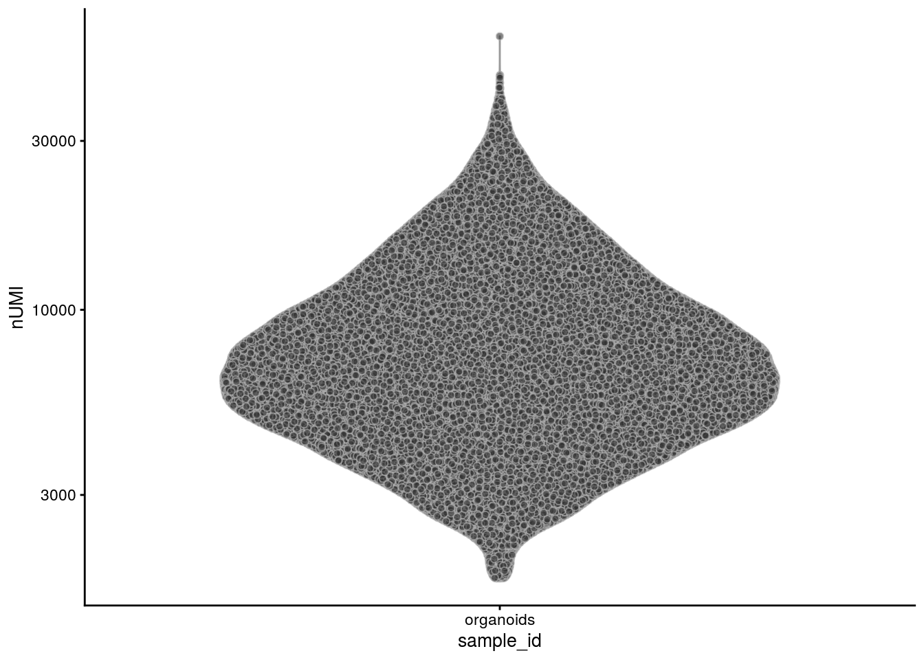
The number of genes:
plotColData(sce, x = "sample_id", y = "nGene") + scale_y_log10() 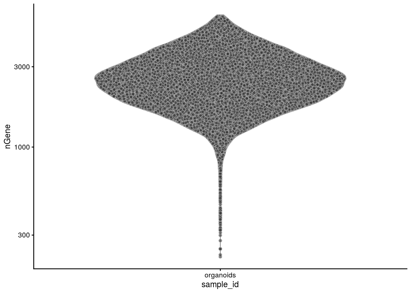
The percentage of mitochondrial genes:
plotColData(sce, x = "sample_id", y = "PercentMito")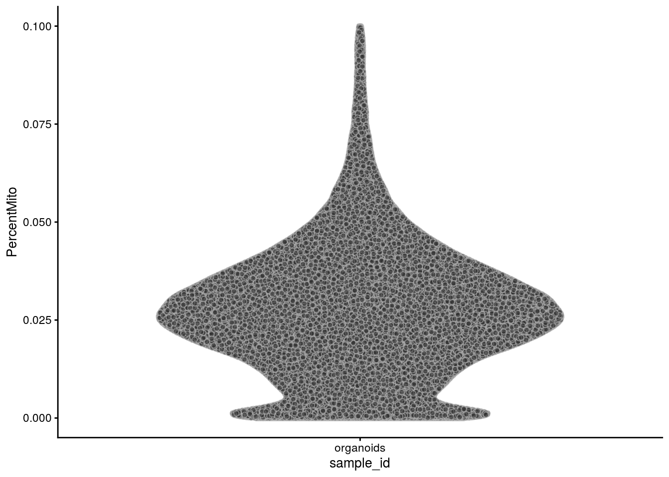
Normalization
We try to recreate Extended Data Fig. 2 a-e.
## subset the cells
sce_all <- sce
sce <- sce[, sce$in_FullLineage]
dim(sce)
[1] 28601 43498# create SeuratObject
so <- CreateSeuratObject(
counts = counts(sce),
meta.data = data.frame(colData(sce)),
project = "organoids")
# split by sample
cells_by_sample <- split(colnames(sce), sce$Sample)
so <- lapply(cells_by_sample, function(i) subset(so, cells = i))
## log normalize the data using a scaling factor of 10000
so <- lapply(so, NormalizeData, verbose = FALSE, scale.factor = 10000,
normalization.method = "LogNormalize")Integration of H9 and 409b2
so_all <- so
sub_samples <- unique(c(colData(sce)[sce$Line %in% c("H9","409b2"),]$Sample))
so <- so[sub_samples]

## Identify the top 2000 genes with high cell-to-cell variation
so <- lapply(so, FindVariableFeatures, nfeatures = 2000,
    selection.method = "vst", verbose = FALSE)
# find anchors & integrate
as <- FindIntegrationAnchors(so, verbose = FALSE)
so <- IntegrateData(anchorset = as, dims = seq_len(20), verbose = FALSE)
#
# ## We scale the data so that mean expression is 0 and variance is 1, across cells
# ## We also regress out the number of UMIs.
# ## We don't have mitochondrial genes for the NES
# DefaultAssay(so) <- "integrated"
so <- ScaleData(so, verbose = FALSE, vars.to.regress = c("nGene", "PercentMito"))Dimension reduction
We perform dimension reduction with t-SNE and UMAP based on PCA results.
so <- RunPCA(so, npcs = 30, verbose = FALSE)
so <- RunTSNE(so, reduction = "pca", dims = seq_len(20),
    seed.use = 1, do.fast = TRUE, verbose = FALSE)
so <- RunUMAP(so, reduction = "pca", dims = seq_len(20),
    seed.use = 1, verbose = FALSE)
Plot PCA results
## PCA plot
DimPlot(so, reduction = "pca", group.by = "sample_id")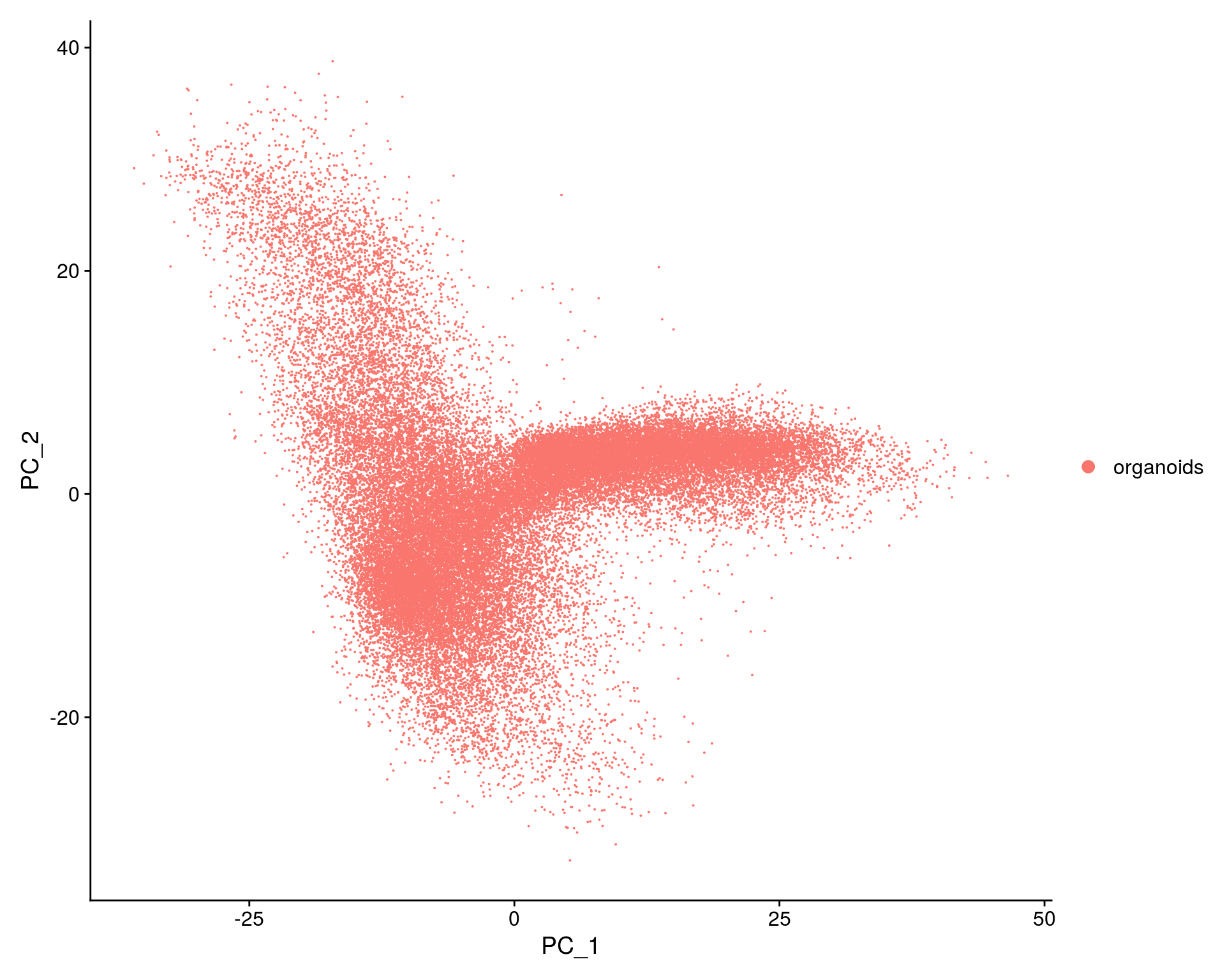
# elbow plot with the ranking of PCs based on the % of variance explained
ElbowPlot(so, ndims = 30)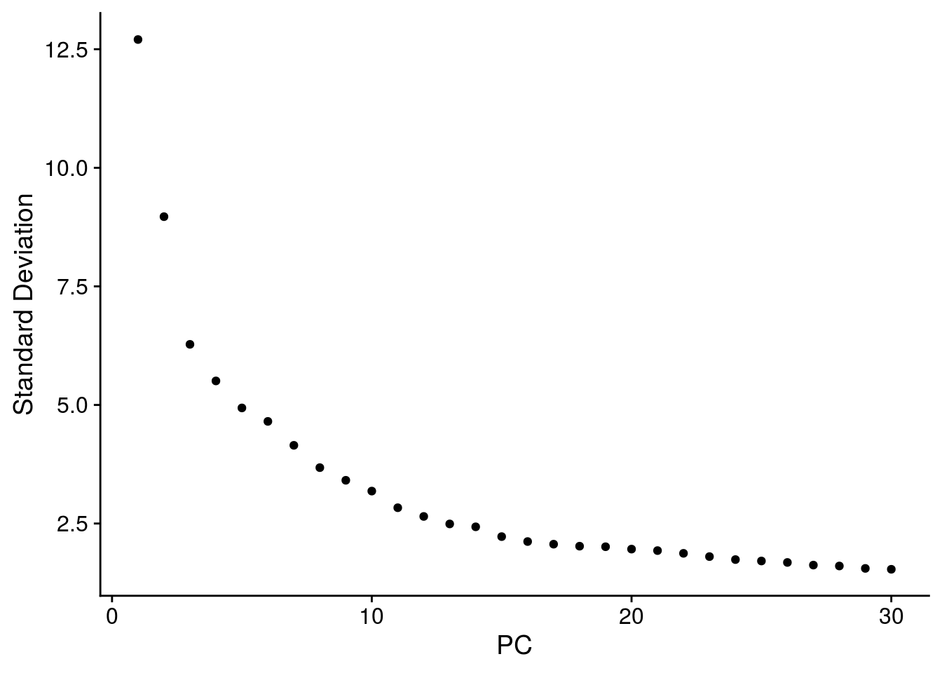
Clustering
We cluster the cells using the reduced PCA dimensions.
so <- FindNeighbors(so, reduction = "pca", dims = seq_len(20), verbose = FALSE)
for (res in c(0.4, 0.6, 0.8))
    so <- FindClusters(so, resolution = res, random.seed = 1, verbose = FALSE)
Dimension reduction plots
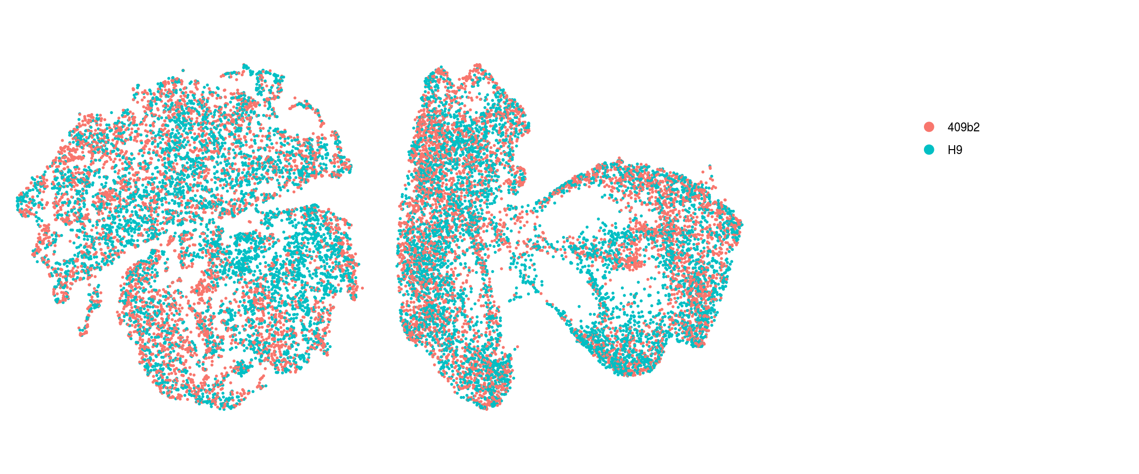
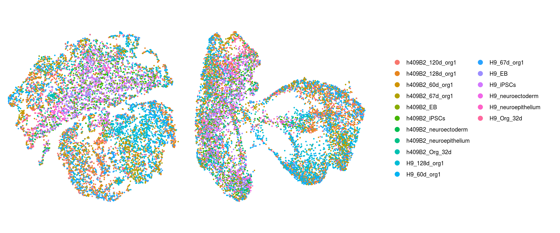
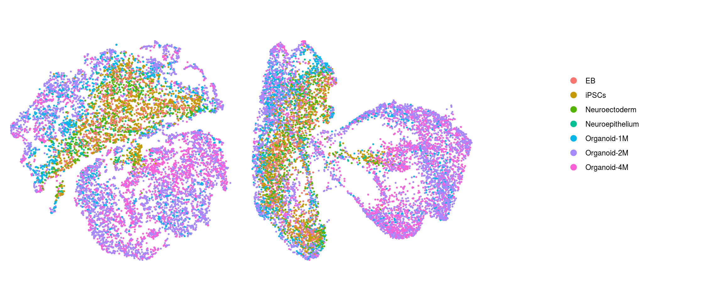
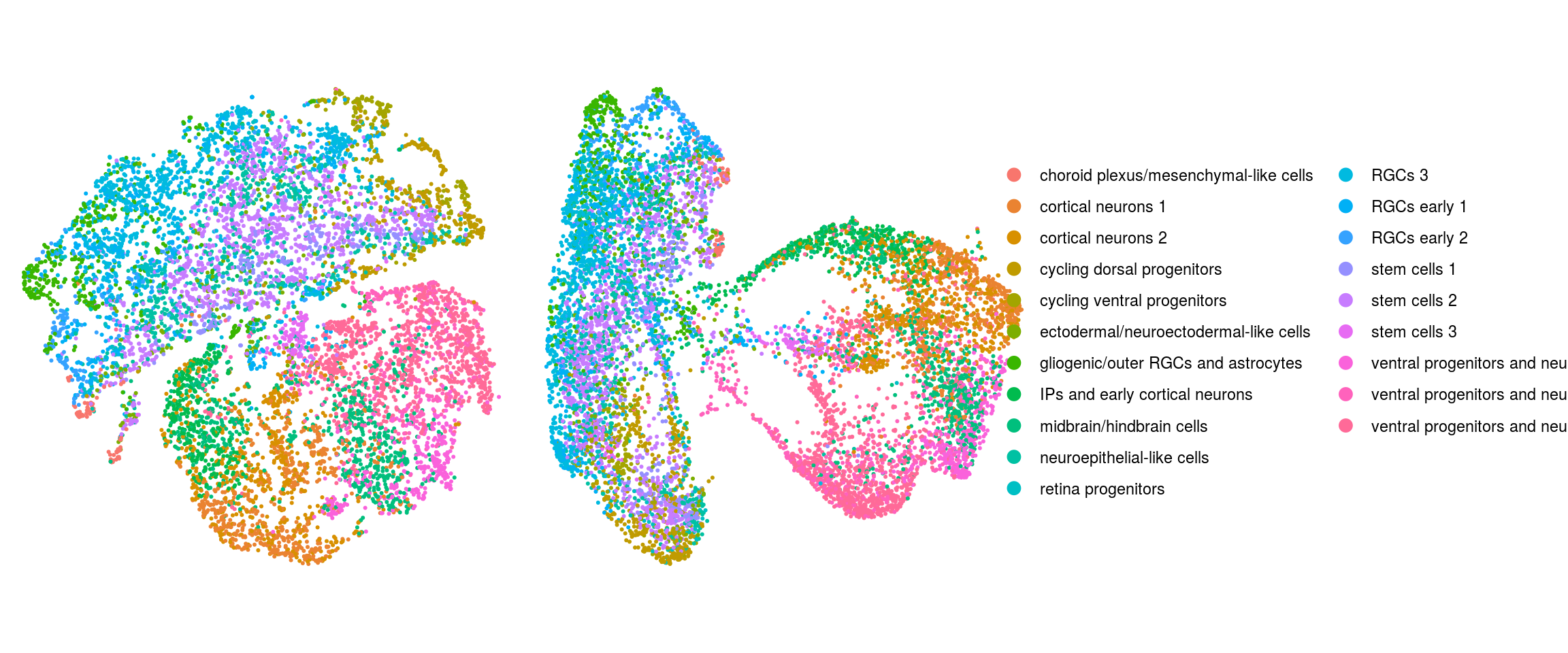
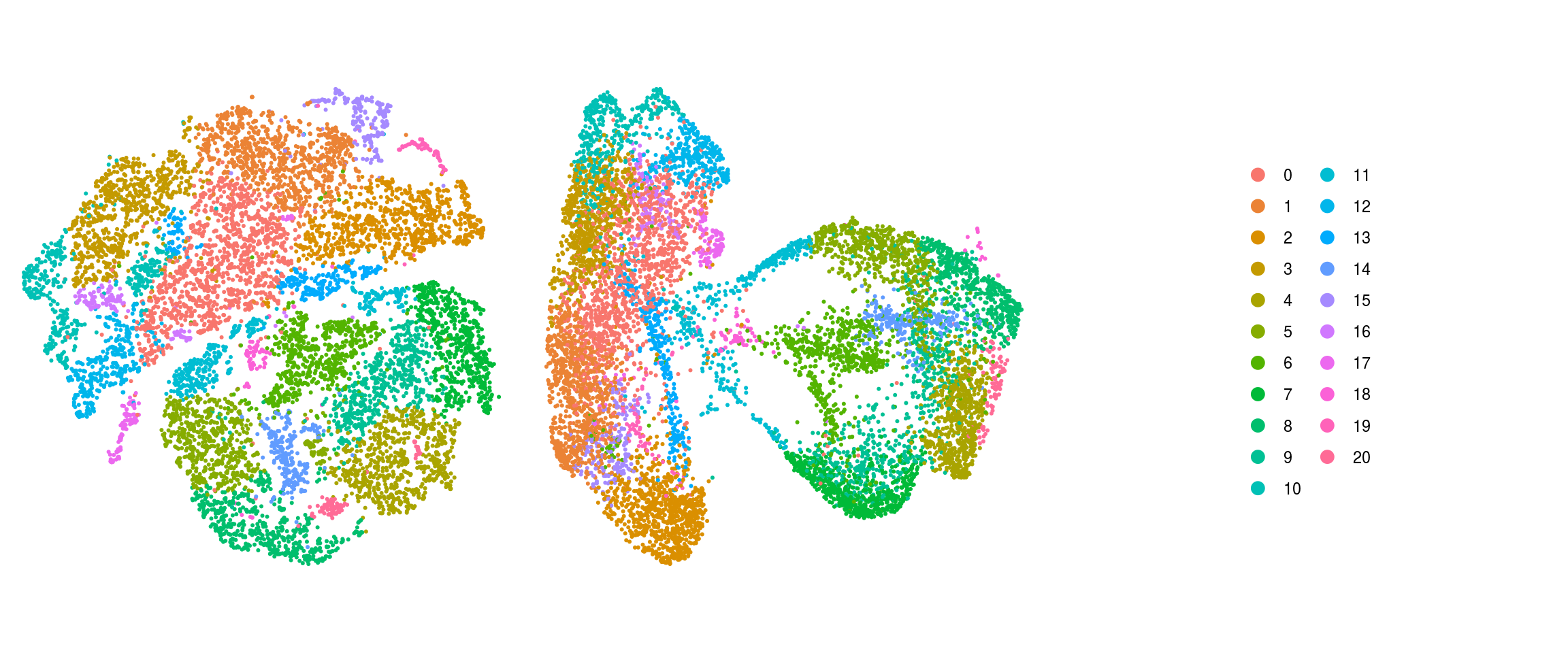
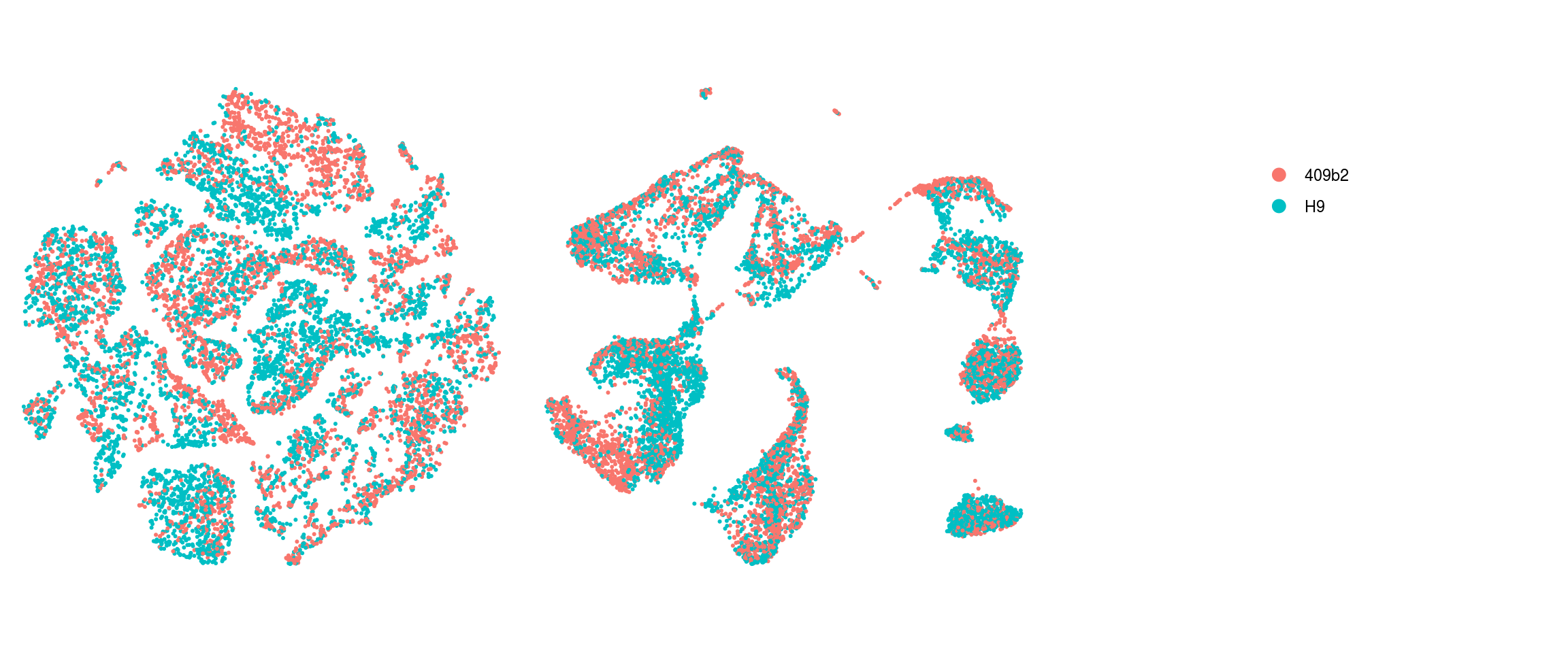
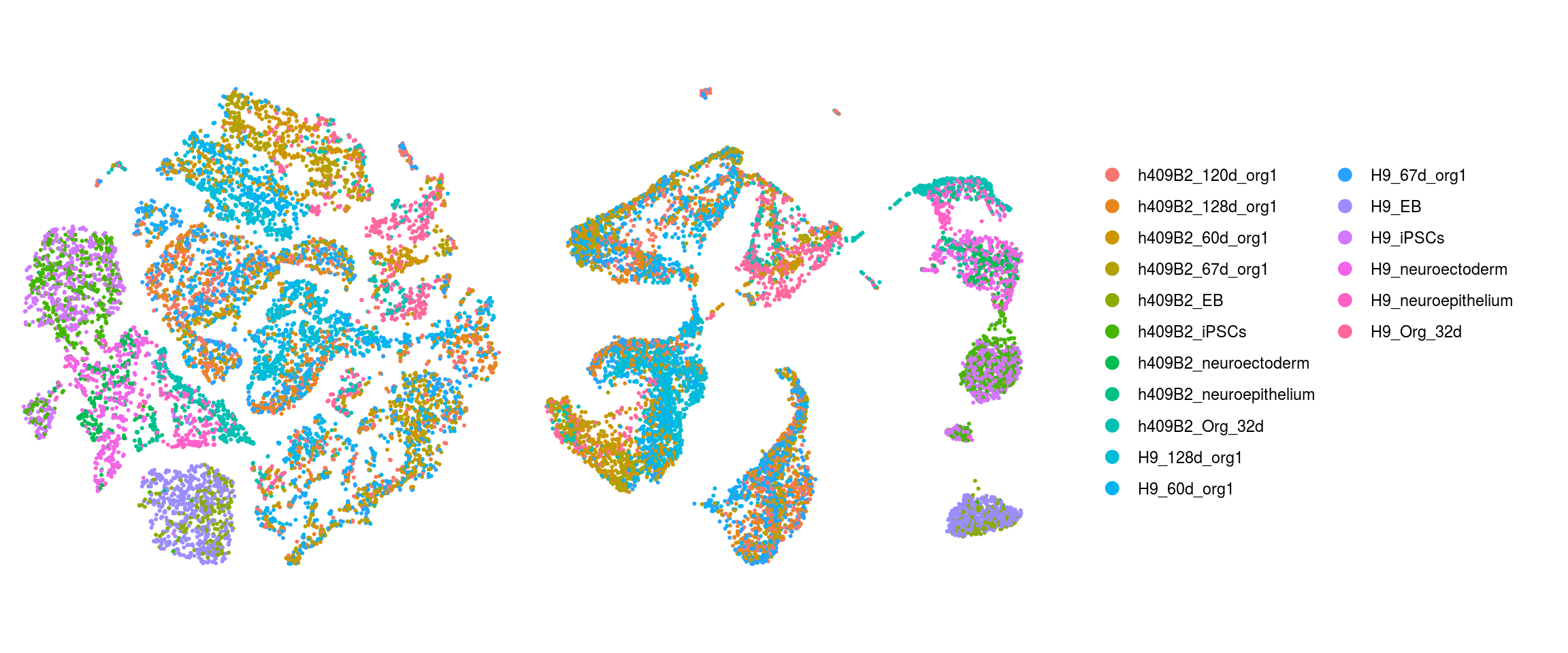
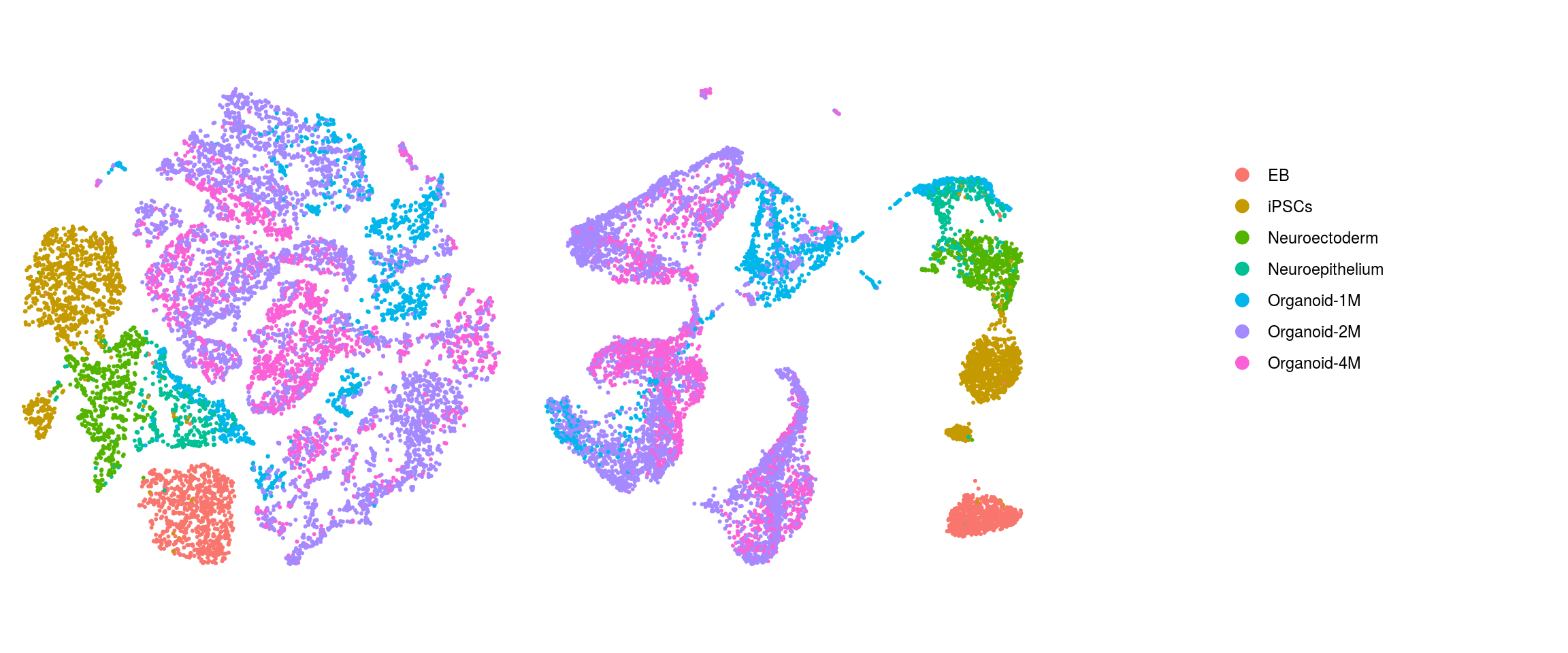
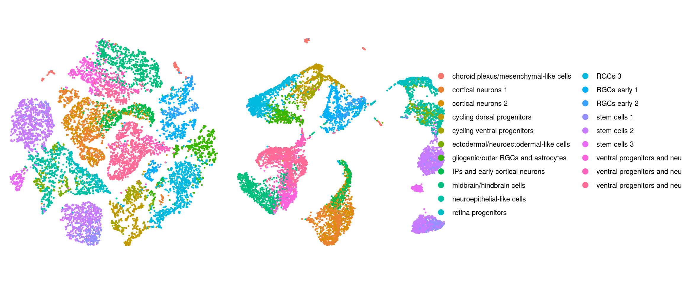
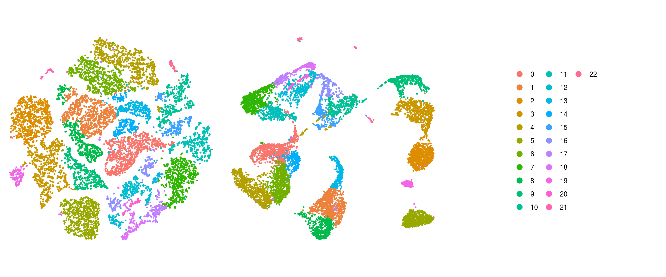
We plot the dimension reduction (DR) and color by cell line, sample, predicted cell type, cluster ID
# set cluster IDs to resolution 0.4 clustering
so <- SetIdent(so, value = "integrated_snn_res.0.6")
so@meta.data$cluster_id <- Idents(so)

cs <- sample(colnames(so), 10e3)
.plot_dr <- function(so, dr, id)
    DimPlot(so, cells = cs, group.by = id, reduction = dr, pt.size = 0.4) +
        guides(col = guide_legend(nrow = 11,
            override.aes = list(size = 3, alpha = 1))) +
        theme_void() + theme(aspect.ratio = 1)
ids <- c("Line", "Sample", "Stage","cl_FullLineage", "ident")
for (id in ids) {
    cat("### ", id, "\n")
    p1 <- .plot_dr(so, "tsne", id)
    lgd <- get_legend(p1)
    p1 <- p1 + theme(legend.position = "none")
    p2 <- .plot_dr(so, "umap", id) + theme(legend.position = "none")
    ps <- plot_grid(plotlist = list(p1, p2), nrow = 1)
    p <- plot_grid(ps, lgd, nrow = 1, rel_widths = c(1, 0.5))
    print(p)
    cat("\n\n")
}
Reproduction of the paper figures
In the paper, the authors used CCA to integrate the H9 and 409b2 cells in a single tSNE plot. We try to use the exact same approach to see if we can reproduce their Extended data figure 2a.
## They describe their pipeline as follows:
## Seurat v3 CCA
## log-normalisation
## highly variable genes with vst (for 409b2 and H9 cells)
## integration using top 20 CCs using the Seurat method by identifying anchors and integrating the datasets
## scale data
## PCA
## clustering based on top 20 PCs, resolution of 0.6
## feature plots with non-integrated expression values

# create SeuratObject for the H9 and 409b2 cells
so <- CreateSeuratObject(
    counts = counts(sce),
    meta.data = data.frame(colData(sce)),
    project = "organoids")

# split by cell line instead of sample as before
cells_by_sample <- split(colnames(sce), sce$Line)
so <- lapply(cells_by_sample, function(i) subset(so, cells = i))

## log normalize the data using a scaling factor of 10000
so <- lapply(so, NormalizeData, verbose = FALSE, scale.factor = 10000,
             normalization.method = "LogNormalize")

## Identify the top 2000 genes with high cell-to-cell variation
so <- lapply(so, FindVariableFeatures, nfeatures = 2000,
    selection.method = "vst", verbose = FALSE)
# find anchors & integrate
as <- FindIntegrationAnchors(so, verbose = FALSE, dims = 1:20)
so <- IntegrateData(anchorset = as, dims = seq_len(20), verbose = FALSE)
# ## We scale the data without regressing out any factors
so <- ScaleData(so, verbose = FALSE)so <- RunPCA(so, npcs = 30, verbose = FALSE)
so <- RunTSNE(so, reduction = "pca", dims = seq_len(20),
seed.use = 1, do.fast = TRUE, verbose = FALSE)
so <- RunUMAP(so, reduction = "pca", dims = seq_len(20),
seed.use = 1, verbose = FALSE)
## PCA plot
DimPlot(so, reduction = "pca", group.by = "sample_id")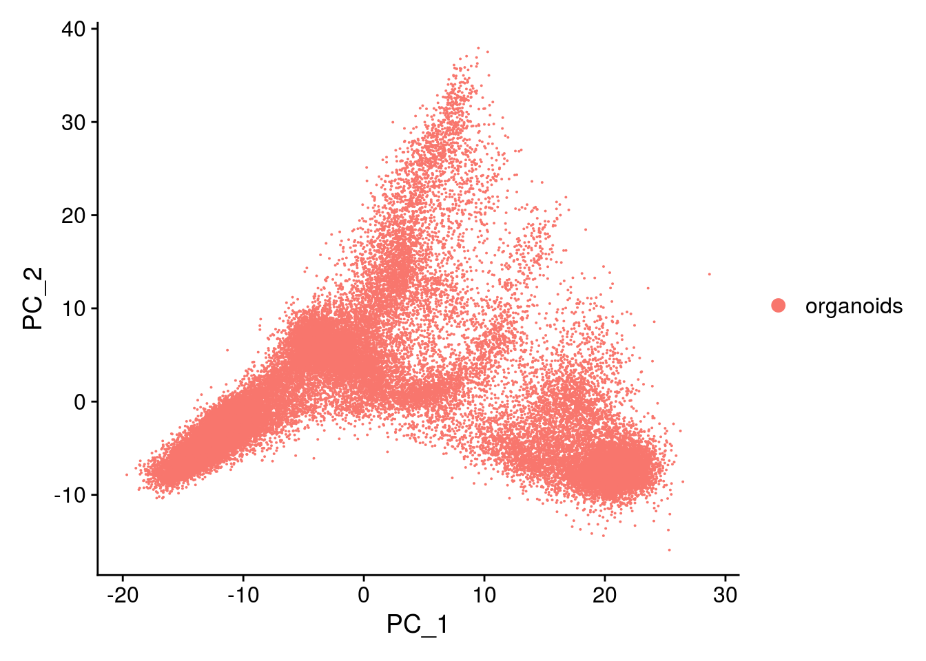
# elbow plot with the ranking of PCs based on the % of variance explained
ElbowPlot(so, ndims = 30)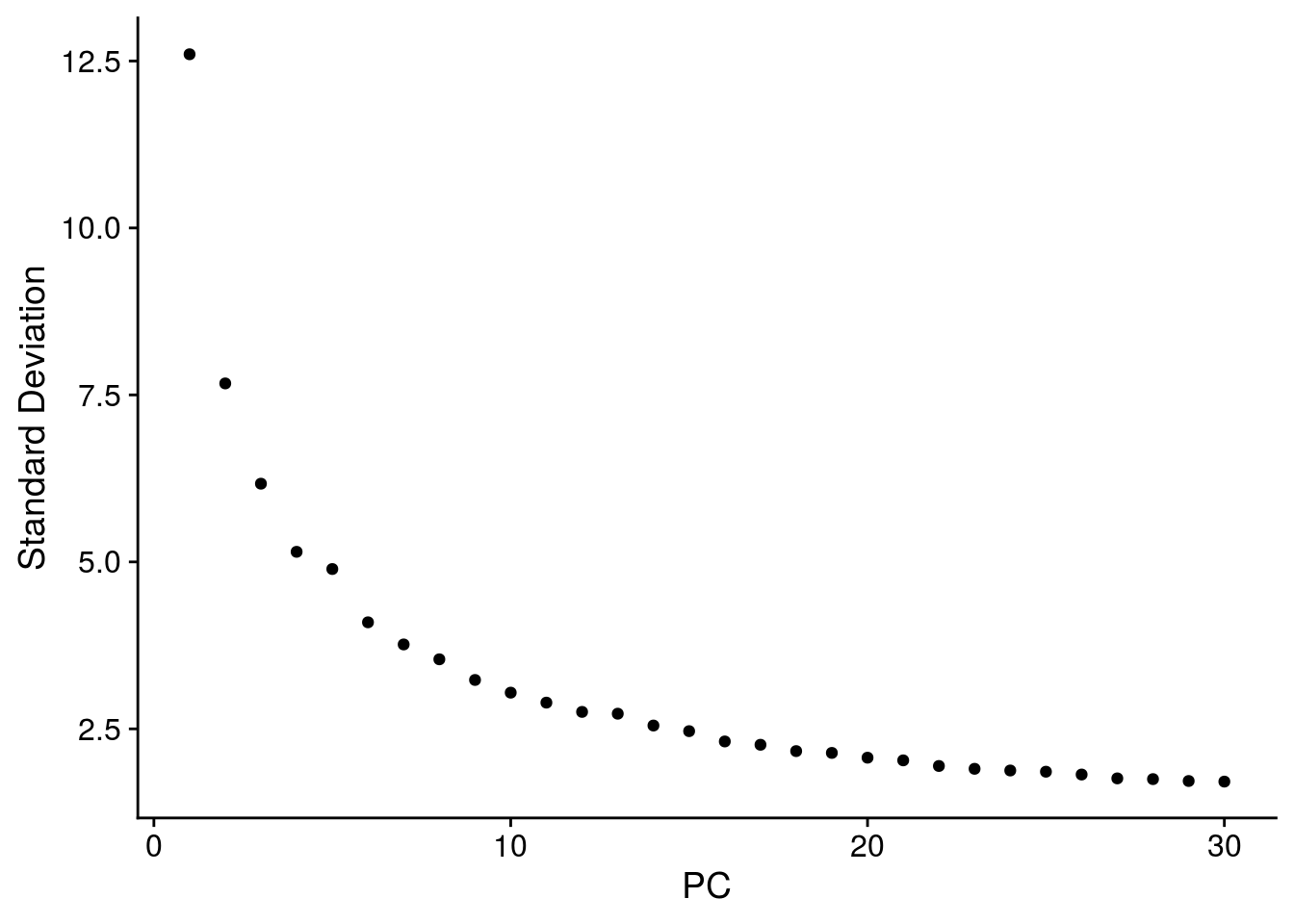
so <- FindNeighbors(so, reduction = "pca", dims = seq_len(20), verbose = FALSE)
so <- FindClusters(so, resolution = 0.6, random.seed = 1, verbose = FALSE)
Dimension reduction plots
We plot the dimension reduction (DR) and color by cell line, sample, predicted cell type, cluster ID
# set cluster IDs to resolution 0.4 clustering
so <- SetIdent(so, value = "integrated_snn_res.0.6")
so@meta.data$cluster_id <- Idents(so)

cs <- sample(colnames(so), 10e3)
.plot_dr <- function(so, dr, id)
    DimPlot(so, cells = cs, group.by = id, reduction = dr, pt.size = 0.4) +
        guides(col = guide_legend(nrow = 11,
            override.aes = list(size = 3, alpha = 1))) +
        theme_void() + theme(aspect.ratio = 1)
ids <- c("Line", "Sample", "Stage","cl_FullLineage", "ident")
for (id in ids) {
    cat("### ", id, "\n")
    p1 <- .plot_dr(so, "tsne", id)
    lgd <- get_legend(p1)
    p1 <- p1 + theme(legend.position = "none")
    p2 <- .plot_dr(so, "umap", id) + theme(legend.position = "none")
    ps <- plot_grid(plotlist = list(p1, p2), nrow = 1)
    p <- plot_grid(ps, lgd, nrow = 1, rel_widths = c(1, 0.5))
    print(p)
    cat("\n\n")
}
Line
Sample
Stage
cl_FullLineage
ident
Save Seurat object to RDS
## Seurat object integrated by sample
saveRDS(so_sample, file.path("output", "so_sample_organoid-01-clustering.rds"))
## Seurat object integrated by cell line
saveRDS(so, file.path("output", "so_organoid-01-clustering.rds"))
saveRDS(sce_all, file.path("output", "sce_organoid-01-clustering.rds"))
sessionInfo()R version 4.0.0 (2020-04-24)
Platform: x86_64-pc-linux-gnu (64-bit)
Running under: Ubuntu 16.04.6 LTS
Matrix products: default
BLAS: /usr/local/R/R-4.0.0/lib/libRblas.so
LAPACK: /usr/local/R/R-4.0.0/lib/libRlapack.so
locale:
[1] LC_CTYPE=en_US.UTF-8 LC_NUMERIC=C
[3] LC_TIME=en_US.UTF-8 LC_COLLATE=en_US.UTF-8
[5] LC_MONETARY=en_US.UTF-8 LC_MESSAGES=en_US.UTF-8
[7] LC_PAPER=en_US.UTF-8 LC_NAME=C
[9] LC_ADDRESS=C LC_TELEPHONE=C
[11] LC_MEASUREMENT=en_US.UTF-8 LC_IDENTIFICATION=C
attached base packages:
[1] parallel stats4 stats graphics grDevices utils datasets
[8] methods base
other attached packages:
[1] data.table_1.12.8 future_1.17.0
[3] rtracklayer_1.48.0 stringr_1.4.0
[5] Seurat_3.1.5 cowplot_1.0.0
[7] dplyr_1.0.0 scater_1.16.2
[9] ggplot2_3.3.2 BiocParallel_1.22.0
[11] scDblFinder_1.2.0 DropletUtils_1.8.0
[13] SingleCellExperiment_1.10.1 SummarizedExperiment_1.18.1
[15] DelayedArray_0.14.0 matrixStats_0.56.0
[17] Biobase_2.48.0 GenomicRanges_1.40.0
[19] GenomeInfoDb_1.24.2 IRanges_2.22.2
[21] S4Vectors_0.26.1 BiocGenerics_0.34.0
[23] workflowr_1.6.2
loaded via a namespace (and not attached):
[1] backports_1.1.8 plyr_1.8.6
[3] igraph_1.2.5 lazyeval_0.2.2
[5] splines_4.0.0 listenv_0.8.0
[7] digest_0.6.25 htmltools_0.5.0
[9] viridis_0.5.1 magrittr_1.5
[11] cluster_2.1.0 ROCR_1.0-11
[13] limma_3.44.3 globals_0.12.5
[15] Biostrings_2.56.0 R.utils_2.9.2
[17] colorspace_1.4-1 rappdirs_0.3.1
[19] ggrepel_0.8.2 xfun_0.15
[21] crayon_1.3.4 RCurl_1.98-1.2
[23] jsonlite_1.7.0 survival_3.2-3
[25] zoo_1.8-8 ape_5.4
[27] glue_1.4.1 gtable_0.3.0
[29] zlibbioc_1.34.0 XVector_0.28.0
[31] leiden_0.3.3 BiocSingular_1.4.0
[33] Rhdf5lib_1.10.0 future.apply_1.6.0
[35] HDF5Array_1.16.1 scales_1.1.1
[37] edgeR_3.30.3 Rcpp_1.0.4.6
[39] viridisLite_0.3.0 reticulate_1.16
[41] dqrng_0.2.1 rsvd_1.0.3
[43] tsne_0.1-3 htmlwidgets_1.5.1
[45] httr_1.4.1 RColorBrewer_1.1-2
[47] ellipsis_0.3.1 ica_1.0-2
[49] farver_2.0.3 pkgconfig_2.0.3
[51] XML_3.99-0.4 R.methodsS3_1.8.0
[53] uwot_0.1.8 locfit_1.5-9.4
[55] labeling_0.3 tidyselect_1.1.0
[57] rlang_0.4.6 reshape2_1.4.4
[59] later_1.1.0.1 munsell_0.5.0
[61] tools_4.0.0 generics_0.0.2
[63] ggridges_0.5.2 evaluate_0.14
[65] yaml_2.2.1 knitr_1.29
[67] fs_1.4.2 fitdistrplus_1.1-1
[69] purrr_0.3.4 randomForest_4.6-14
[71] RANN_2.6.1 pbapply_1.4-2
[73] nlme_3.1-148 whisker_0.4
[75] scran_1.16.0 R.oo_1.23.0
[77] compiler_4.0.0 beeswarm_0.2.3
[79] plotly_4.9.2.1 png_0.1-7
[81] tibble_3.0.1 statmod_1.4.34
[83] stringi_1.4.6 RSpectra_0.16-0
[85] lattice_0.20-41 Matrix_1.2-18
[87] vctrs_0.3.1 pillar_1.4.4
[89] lifecycle_0.2.0 lmtest_0.9-37
[91] RcppAnnoy_0.0.16 BiocNeighbors_1.6.0
[93] bitops_1.0-6 irlba_2.3.3
[95] httpuv_1.5.4 patchwork_1.0.1
[97] R6_2.4.1 promises_1.1.1
[99] KernSmooth_2.23-17 gridExtra_2.3
[101] vipor_0.4.5 codetools_0.2-16
[103] MASS_7.3-51.6 rhdf5_2.32.2
[105] rprojroot_1.3-2 withr_2.2.0
[107] GenomicAlignments_1.24.0 Rsamtools_2.4.0
[109] sctransform_0.2.1 GenomeInfoDbData_1.2.3
[111] grid_4.0.0 tidyr_1.1.0
[113] rmarkdown_2.3 DelayedMatrixStats_1.10.1
[115] Rtsne_0.15 git2r_0.27.1
[117] ggbeeswarm_0.6.0