Integration NSC from Lam et al.
Katharina Hembach
7/3/2020
Last updated: 2020-07-10
Checks: 7 0
Knit directory: neural_scRNAseq/
This reproducible R Markdown analysis was created with workflowr (version 1.6.2). The Checks tab describes the reproducibility checks that were applied when the results were created. The Past versions tab lists the development history.
Great! Since the R Markdown file has been committed to the Git repository, you know the exact version of the code that produced these results.
Great job! The global environment was empty. Objects defined in the global environment can affect the analysis in your R Markdown file in unknown ways. For reproduciblity it's best to always run the code in an empty environment.
The command set.seed(20200522) was run prior to running the code in the R Markdown file. Setting a seed ensures that any results that rely on randomness, e.g. subsampling or permutations, are reproducible.
Great job! Recording the operating system, R version, and package versions is critical for reproducibility.
Nice! There were no cached chunks for this analysis, so you can be confident that you successfully produced the results during this run.
Great job! Using relative paths to the files within your workflowr project makes it easier to run your code on other machines.
Great! You are using Git for version control. Tracking code development and connecting the code version to the results is critical for reproducibility.
The results in this page were generated with repository version 15a0ad2. See the Past versions tab to see a history of the changes made to the R Markdown and HTML files.
Note that you need to be careful to ensure that all relevant files for the analysis have been committed to Git prior to generating the results (you can use wflow_publish or wflow_git_commit). workflowr only checks the R Markdown file, but you know if there are other scripts or data files that it depends on. Below is the status of the Git repository when the results were generated:
Ignored files:
    Ignored:    .DS_Store
    Ignored:    .Rhistory
    Ignored:    .Rproj.user/
    Ignored:    ._.DS_Store
    Ignored:    ._Rplots.pdf
    Ignored:    .__workflowr.yml
    Ignored:    ._neural_scRNAseq.Rproj
    Ignored:    analysis/.DS_Store
    Ignored:    analysis/.Rhistory
    Ignored:    analysis/._.DS_Store
    Ignored:    analysis/._01-preprocessing.Rmd
    Ignored:    analysis/._01-preprocessing.html
    Ignored:    analysis/._02.1-SampleQC.Rmd
    Ignored:    analysis/._03-filtering.Rmd
    Ignored:    analysis/._04-clustering.Rmd
    Ignored:    analysis/._04-clustering.knit.md
    Ignored:    analysis/._04.1-cell_cycle.Rmd
    Ignored:    analysis/._05-annotation.Rmd
    Ignored:    analysis/._Lam-0-NSC_no_integration.Rmd
    Ignored:    analysis/._Lam-01-NSC_integration.Rmd
    Ignored:    analysis/._Lam-02-NSC_annotation.Rmd
    Ignored:    analysis/._NSC-1-clustering.Rmd
    Ignored:    analysis/._NSC-2-annotation.Rmd
    Ignored:    analysis/.__site.yml
    Ignored:    analysis/._additional_filtering.Rmd
    Ignored:    analysis/._additional_filtering_clustering.Rmd
    Ignored:    analysis/._index.Rmd
    Ignored:    analysis/01-preprocessing_cache/
    Ignored:    analysis/02-1-SampleQC_cache/
    Ignored:    analysis/02-quality_control_cache/
    Ignored:    analysis/02.1-SampleQC_cache/
    Ignored:    analysis/03-filtering_cache/
    Ignored:    analysis/04-clustering_cache/
    Ignored:    analysis/04.1-cell_cycle_cache/
    Ignored:    analysis/05-annotation_cache/
    Ignored:    analysis/Lam-02-NSC_annotation_cache/
    Ignored:    analysis/NSC-1-clustering_cache/
    Ignored:    analysis/NSC-2-annotation_cache/
    Ignored:    analysis/additional_filtering_cache/
    Ignored:    analysis/additional_filtering_clustering_cache/
    Ignored:    analysis/sample5_QC_cache/
    Ignored:    data/.DS_Store
    Ignored:    data/._.DS_Store
    Ignored:    data/._.smbdeleteAAA17ed8b4b
    Ignored:    data/._Lam_figure2_markers.R
    Ignored:    data/._known_NSC_markers.R
    Ignored:    data/._known_cell_type_markers.R
    Ignored:    data/._metadata.csv
    Ignored:    data/data_sushi/
    Ignored:    data/filtered_feature_matrices/
    Ignored:    output/.DS_Store
    Ignored:    output/._.DS_Store
    Ignored:    output/Lam-01-clustering.rds
    Ignored:    output/NSC_1_clustering.rds
    Ignored:    output/additional_filtering.rds
    Ignored:    output/figures/
    Ignored:    output/sce_01_preprocessing.rds
    Ignored:    output/sce_02_quality_control.rds
    Ignored:    output/sce_03_filtering.rds
    Ignored:    output/sce_preprocessing.rds
    Ignored:    output/so_04_1_cell_cycle.rds
    Ignored:    output/so_04_clustering.rds
    Ignored:    output/so_additional_filtering_clustering.rds

Untracked files:
    Untracked:  Rplots.pdf
    Untracked:  analysis/Lam-0-NSC_no_integration.Rmd
    Untracked:  analysis/additional_filtering.Rmd
    Untracked:  analysis/additional_filtering_clustering.Rmd
    Untracked:  analysis/sample5_QC.Rmd
    Untracked:  data/Homo_sapiens.GRCh38.98.sorted.gtf
    Untracked:  data/Lam_et_al/
    Untracked:  scripts/

Unstaged changes:
    Modified:   analysis/_site.yml
    Modified:   data/Lam_figure2_markers.R
Note that any generated files, e.g. HTML, png, CSS, etc., are not included in this status report because it is ok for generated content to have uncommitted changes.
These are the previous versions of the repository in which changes were made to the R Markdown (analysis/Lam-01-NSC_integration.Rmd) and HTML (docs/Lam-01-NSC_integration.html) files. If you've configured a remote Git repository (see ?wflow_git_remote), click on the hyperlinks in the table below to view the files as they were in that past version.
| File | Version | Author | Date | Message |
|---|---|---|---|---|
| Rmd | 15a0ad2 | khembach | 2020-07-10 | compare cell cluster membership before and after NES integration; merge |
| html | a1ebb78 | khembach | 2020-07-08 | Build site. |
| Rmd | d8bd339 | khembach | 2020-07-08 | NSC integration with NES from Lam et al. |
Load packages
library(cowplot)
library(ggplot2)
library(Seurat)
library(SingleCellExperiment)
library(stringr)
library(Seurat)
library(rtracklayer)
library(future)
library(biomaRt)
library(dplyr)
library(data.table)
library(ComplexHeatmap)
library(RColorBrewer)
# increase future's maximum allowed size of exported globals to 4GB
# the default is 2GB
options(future.globals.maxSize = 4096 * 1024 ^ 2)
# change the current plan to access parallelization
plan("multiprocess", workers = 20)Load our NSC data
# sce <- readRDS(file.path("output", "sce_03_filtering.rds"))
## our NSC from sample 1 and 2
# so <- readRDS(file.path("output", "NSC_1_clustering.rds"))

sce <- readRDS(file.path("output", "sce_03_filtering.rds"))

## subset the two NSC samples
sce <- sce[,colData(sce)$sample_id %in% c("1NSC", "2NSC")]
sce$sample_id <- droplevels(sce$sample_id)
# ## we filter genes and require > 1 count in at least 20 cells
# sce <- sce[rowSums(counts(sce) > 1) >= 20, ]
# dim(sce)

# create SeuratObject
so <- CreateSeuratObject(
    counts = counts(sce),
    meta.data = data.frame(colData(sce)),
    project = "neural_cultures")
Load NES data and map symbol to Ensembl IDs
nes_meta <- read.table(file.path("data", "Lam_et_al", "figure2", "Figure_2_metadata.NES.Healthy.Cell.lines.healthy_NES.7.clusters.final.figure.txt"))

nes_counts <- read.table(file.path("data", "Lam_et_al", "figure2", "Figure_2_NES.Healthy.Cell.lines.healthy_NES.7.clusters.final.figure.txt"))

sce_nes <- SingleCellExperiment(list(counts=nes_counts), colData = nes_meta)
dim(sce_nes)
[1] 14086 768## I think Lam et al. used UCSC hg19 gene annotations for their analysis.
## --> we map the gene symbols to hg19 Ensembl IDs
grch37 <- biomaRt::useMart(biomart="ENSEMBL_MART_ENSEMBL", host="grch37.ensembl.org",
path="/biomart/martservice", dataset="hsapiens_gene_ensembl")
res <- getBM(attributes=c('hgnc_symbol', 'ensembl_gene_id'),
filters = 'hgnc_symbol',
values = rownames(sce_nes),
mart = grch37)
table(rownames(sce_nes) %in% res$hgnc_symbol)
FALSE  TRUE
 1450 12636
res_split <- split(res$ensembl_gene_id, res$hgnc_symbol)
# we match our Ensembl IDs to the biomaRt IDs and only keep rows from Lam et al.
# that match one of our IDs
a <- res %>% dplyr::left_join(data.frame(rowData(sce)),
by = c("ensembl_gene_id" = "ensembl_id"))
## if a symbols has multiple IDs, we keep the ID with the same symbol in our dataset
## find all duplicates
dups <- duplicated(a$hgnc_symbol) | duplicated(a$hgnc_symbol, fromLast=TRUE)
## check the symbol in our dataset and remove the duplicate with wrong symbol
b_split <- split(a[dups,], a[dups,]$hgnc_symbol)
## if GRCh38 symbol matches the hgnc_symbol, we keep the corresponding Ensembl ID
## otherwise we only keep the gene symbol without an ID
resolve_dups <- function(b){
res <- b[which(b$hgnc_symbol == b$symbol),]
if (nrow(res) != 1){
res <- b[1,]
res[, c("ensembl_gene_id", "symbol")] <- ""
}
res
}
b_resolved <- lapply(b_split, resolve_dups)
b_resolved <- rbindlist(b_resolved)
id_map <- rbind(a[!dups,], b_resolved)
id_map$symbol <- NULL
colnames(id_map) <- c("symbol", "ensembl_id")
## Remove the features for which we don't have an ensembl ID
sce_nes <- sce_nes[rownames(sce_nes) %in% id_map$symbol,]
dim(sce_nes)[1] 12636 768## We have to use identical gene symbols for all datasets if we want to integrate the data.
## We replace the Lam et al. gene symbols with GRCh38 symbols for all features
## where the Ensembl IDs could be mapped.
gtf <- import(file.path("data", "Homo_sapiens.GRCh38.98.sorted.gtf"))
gene <- gtf[gtf$type == "gene"]
m <- match(id_map$symbol, gene$gene_name)
id_map[!is.na(m),]$symbol <- gene$gene_name[m[!is.na(m)]]
## adjust row and colData
colData(sce_nes)$sample_id <- factor("NES")
rowData(sce_nes) <- id_map[match(rownames(sce_nes), id_map$symbol),]
rownames(sce_nes) <- with(rowData(sce_nes),
paste(ensembl_id, symbol, sep = "."))
sce_nes$group_id <- "NES"
## how many genes could be mapped between datasets?
rownames(sce_nes) %in% rownames(sce) %>% table.
FALSE TRUE
1867 10769 ## The data already comes with the number of RNAs and features
names(colData(sce_nes))[names(colData(sce_nes)) == 'BARCODE'] <- 'barcode'
names(colData(sce_nes))[names(colData(sce_nes)) == 'nCount_RNA'] <- 'sum'
names(colData(sce_nes))[names(colData(sce_nes)) == 'nFeature_RNA'] <- 'detected'
# ## we filter genes and require > 1 count in at least 5 cells
# sce_nes <- sce_nes[rowSums(counts(sce_nes) > 1) >= 5, ]
# dim(sce_nes)
## Only keep the features that are measured in both data sets
sce_nes <- sce_nes[rownames(sce_nes) %in% rownames(sce),]
sce <- sce[rownames(sce) %in% rownames(sce_nes),]
so_nes <- CreateSeuratObject(
counts = counts(sce_nes),
meta.data = data.frame(colData(sce_nes)),
project = "neural_cultures")Clustering before integration
We identify variable features and run PCA, followed by UMAP and clustering without integration. We want to know if there are big differences between the two datasets that make an integration necessary.
## combined Seurat object with both datasets
m <- match(rownames(sce_nes), rownames(sce))
counts <- DelayedArray::cbind(counts(sce), DelayedArray(counts(sce_nes)[m,]))
cdata <- colData(sce) %>% data.frame %>%
  mutate(rownames = rownames(colData(sce))) %>%
  dplyr::full_join(colData(sce_nes) %>%
                     data.frame %>%
                     mutate(rownames = rownames(colData(sce_nes))))
rownames(cdata) <- cdata$rownames
cdata$rownames <- NULL

so <- CreateSeuratObject(
    counts = counts,
    meta.data = cdata,
    project = "neural_cultures")

so <- NormalizeData(so, verbose = FALSE, scale.factor = 10000,
                    normalization.method = "LogNormalize")

so <- FindVariableFeatures(so, nfeatures = 2000,
    selection.method = "vst", verbose = FALSE)
so <- ScaleData(so, verbose = FALSE, vars.to.regress = "sum")

so <- RunPCA(so, npcs = 30, verbose = FALSE)
so <- RunTSNE(so, reduction = "pca", dims = seq_len(20),
    seed.use = 1, do.fast = TRUE, verbose = FALSE)
so <- RunUMAP(so, reduction = "pca", dims = seq_len(20),
    seed.use = 1, verbose = FALSE)
Warning: The default method for RunUMAP has changed from calling Python UMAP via reticulate to the R-native UWOT using the cosine metric
To use Python UMAP via reticulate, set umap.method to 'umap-learn' and metric to 'correlation'
This message will be shown once per sessionDimPlot(so, reduction = "pca", group.by = "sample_id")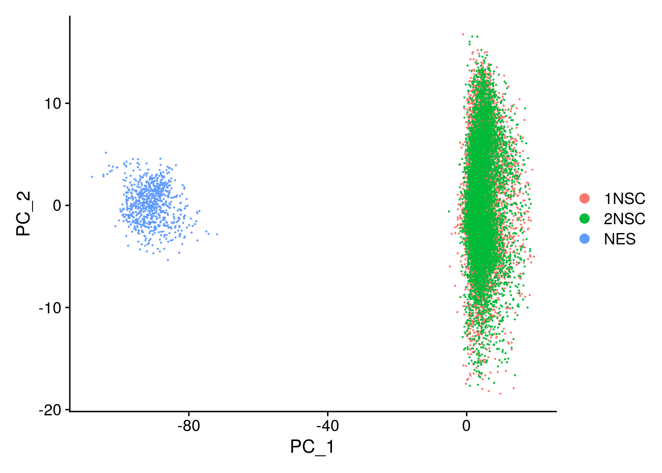
so <- FindNeighbors(so, reduction = "pca", dims = seq_len(20), verbose = FALSE)
so <- FindClusters(so, resolution = 0.4, random.seed = 1, verbose = FALSE)

thm <- theme(aspect.ratio = 1, legend.position = "none")
ps <- lapply(c("sample_id", "group_id", "ident"), function(u) {
    p1 <- DimPlot(so, reduction = "tsne", group.by = u) + thm
    p2 <- DimPlot(so, reduction = "umap", group.by = u)
    lgd <- get_legend(p2)
    p2 <- p2 + thm
    list(p1, p2, lgd)
    plot_grid(p1, p2, lgd, nrow = 1,
        rel_widths = c(1, 1, 0.5))
})
plot_grid(plotlist = ps, ncol = 1)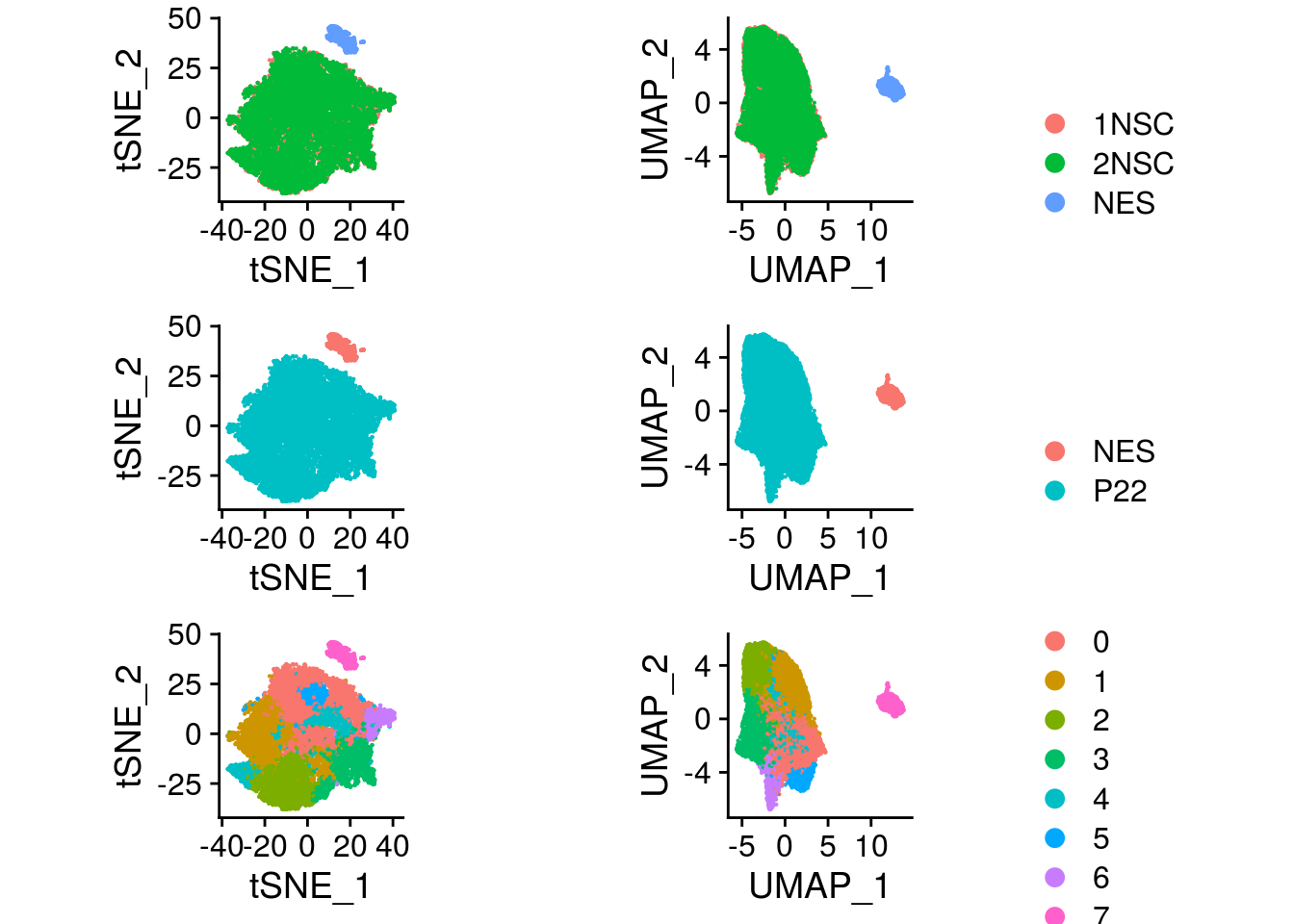
The NES cells cluster apart from our NSCs and we need to integrate the datasets.
Integrated analysis
Now we repeat the clustering on the integrated data.
Normalisation
# split by sample
cells_by_sample <- split(colnames(sce), sce$sample_id)
so <- lapply(cells_by_sample, function(i) subset(so, cells = i))
## add the NES
so[["NES"]] <- so_nes

## log normalize the data using a scaling factor of 10000
so <- lapply(so, NormalizeData, verbose = FALSE, scale.factor = 10000,
             normalization.method = "LogNormalize")
## Identify the top 2000 genes with high cell-to-cell variation
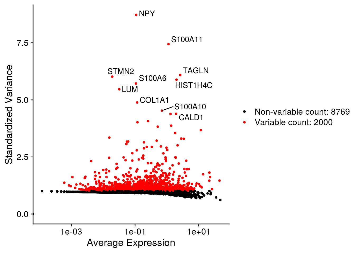
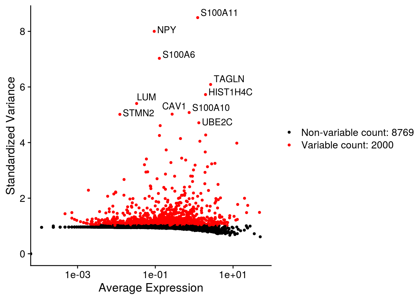
so <- lapply(so, FindVariableFeatures, nfeatures = 2000,
selection.method = "vst", verbose = FALSE)
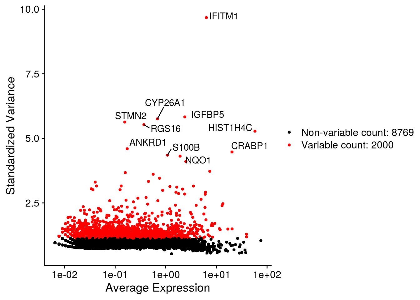
## Plot variable features
for (i in names(so)) {
# Identify the 10 most highly variable genes
top10 <- head(VariableFeatures(so[[i]]), 10)
p <- VariableFeaturePlot(so[[i]])
p <- LabelPoints(plot = p, points = top10,
labels = str_split(top10, "\\.", simplify = TRUE)[,2],
repel = TRUE)
print(p)
}
| Version | Author | Date |
|---|---|---|
| a1ebb78 | khembach | 2020-07-08 |
| Version | Author | Date |
|---|---|---|
| a1ebb78 | khembach | 2020-07-08 |
| Version | Author | Date |
|---|---|---|
| a1ebb78 | khembach | 2020-07-08 |
# find anchors & integrate
as <- FindIntegrationAnchors(so, verbose = FALSE)
so <- IntegrateData(anchorset = as, dims = seq_len(30), verbose = FALSE)

## We scale the data so that mean expression is 0 and variance is 1, across cells
## We also regress out the number of UMIs.
## We don't have mitochondrial genes for the NES
DefaultAssay(so) <- "integrated"
so <- ScaleData(so, verbose = FALSE, vars.to.regress = "sum")
Dimension reduction
We perform dimension reduction with t-SNE and UMAP based on PCA results.
so <- RunPCA(so, npcs = 30, verbose = FALSE)
so <- RunTSNE(so, reduction = "pca", dims = seq_len(20),
    seed.use = 1, do.fast = TRUE, verbose = FALSE)
so <- RunUMAP(so, reduction = "pca", dims = seq_len(20),
    seed.use = 1, verbose = FALSE)
Plot PCA results
# top genes that are associated with the first two PCs
VizDimLoadings(so, dims = 1:2, reduction = "pca")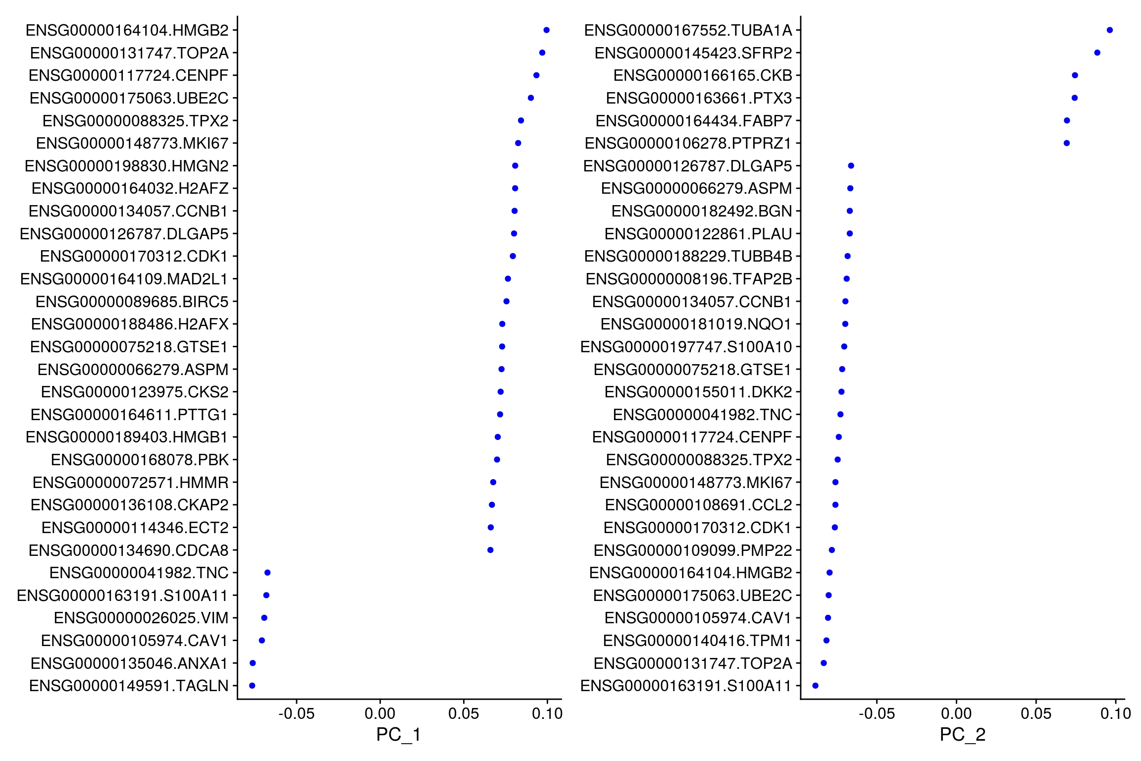
| Version | Author | Date |
|---|---|---|
| a1ebb78 | khembach | 2020-07-08 |
## PCA plot
DimPlot(so, reduction = "pca", group.by = "sample_id")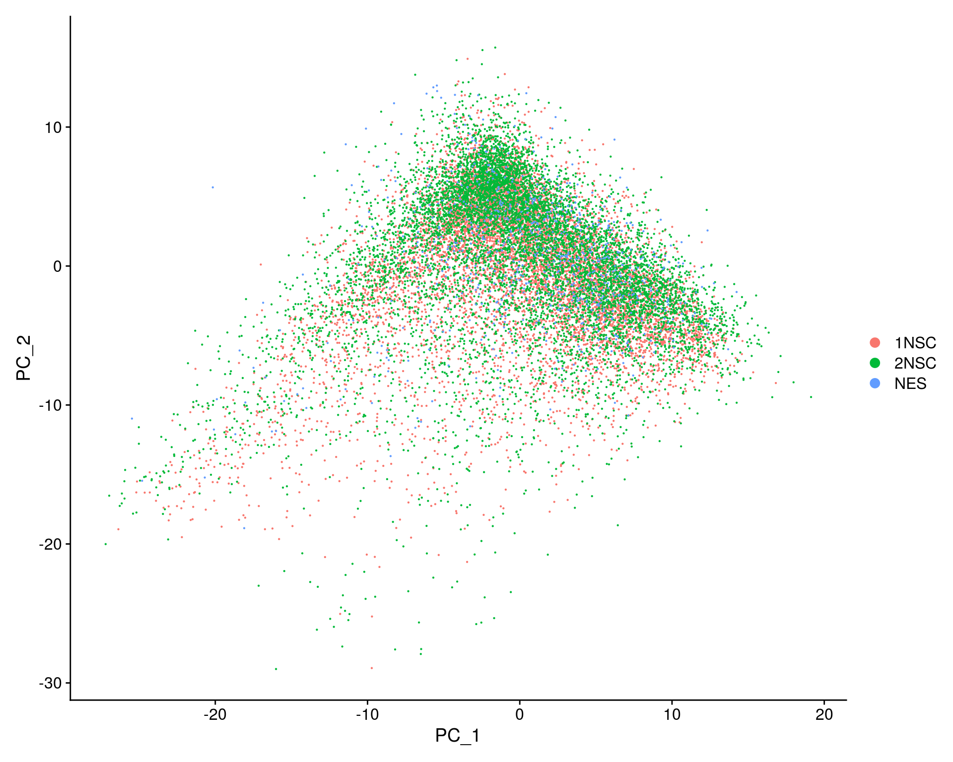
| Version | Author | Date |
|---|---|---|
| a1ebb78 | khembach | 2020-07-08 |
# elbow plot with the ranking of PCs based on the % of variance explained
ElbowPlot(so, ndims = 30)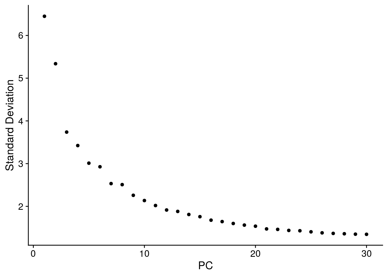
| Version | Author | Date |
|---|---|---|
| a1ebb78 | khembach | 2020-07-08 |
## heatmaps of the top 20 PCs and the 500 most extreme cells for each component
DimHeatmap(so, dims = 1:20, cells = 500, balanced = TRUE, nfeatures = 20 )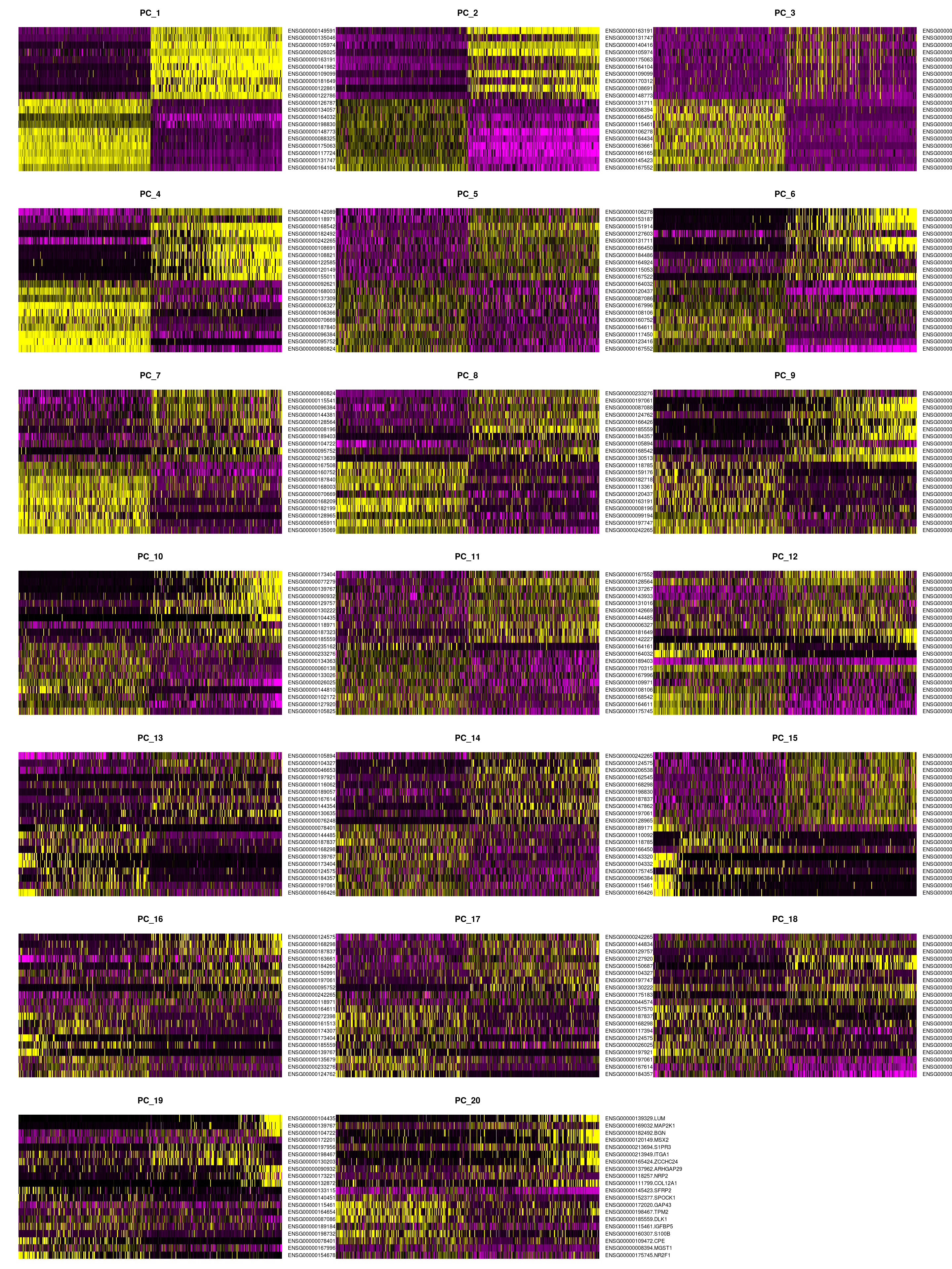
| Version | Author | Date |
|---|---|---|
| a1ebb78 | khembach | 2020-07-08 |
Clustering
We cluster the cells using the reduced PCA dimensions.
so <- FindNeighbors(so, reduction = "pca", dims = seq_len(20), verbose = FALSE)
for (res in c(0.1, 0.2, 0.4, 0.8, 1, 1.2, 2))
    so <- FindClusters(so, resolution = res, random.seed = 1, verbose = FALSE)
Dimension reduction plots
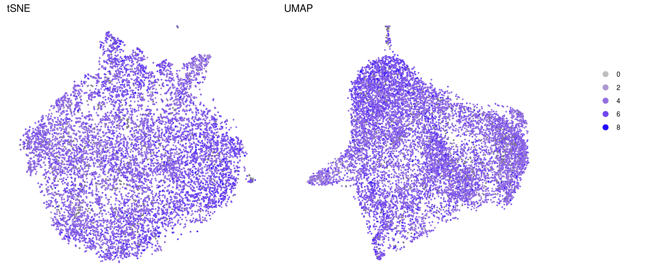
We plot the dimension reduction (DR) and color by sample, group and cluster ID
thm <- theme(aspect.ratio = 1, legend.position = "none")
ps <- lapply(c("sample_id", "group_id", "ident"), function(u) {
    p1 <- DimPlot(so, reduction = "tsne", group.by = u) + thm
    p2 <- DimPlot(so, reduction = "umap", group.by = u)
    lgd <- get_legend(p2)
    p2 <- p2 + thm
    list(p1, p2, lgd)
    plot_grid(p1, p2, lgd, nrow = 1,
        rel_widths = c(1, 1, 0.5))
})
plot_grid(plotlist = ps, ncol = 1)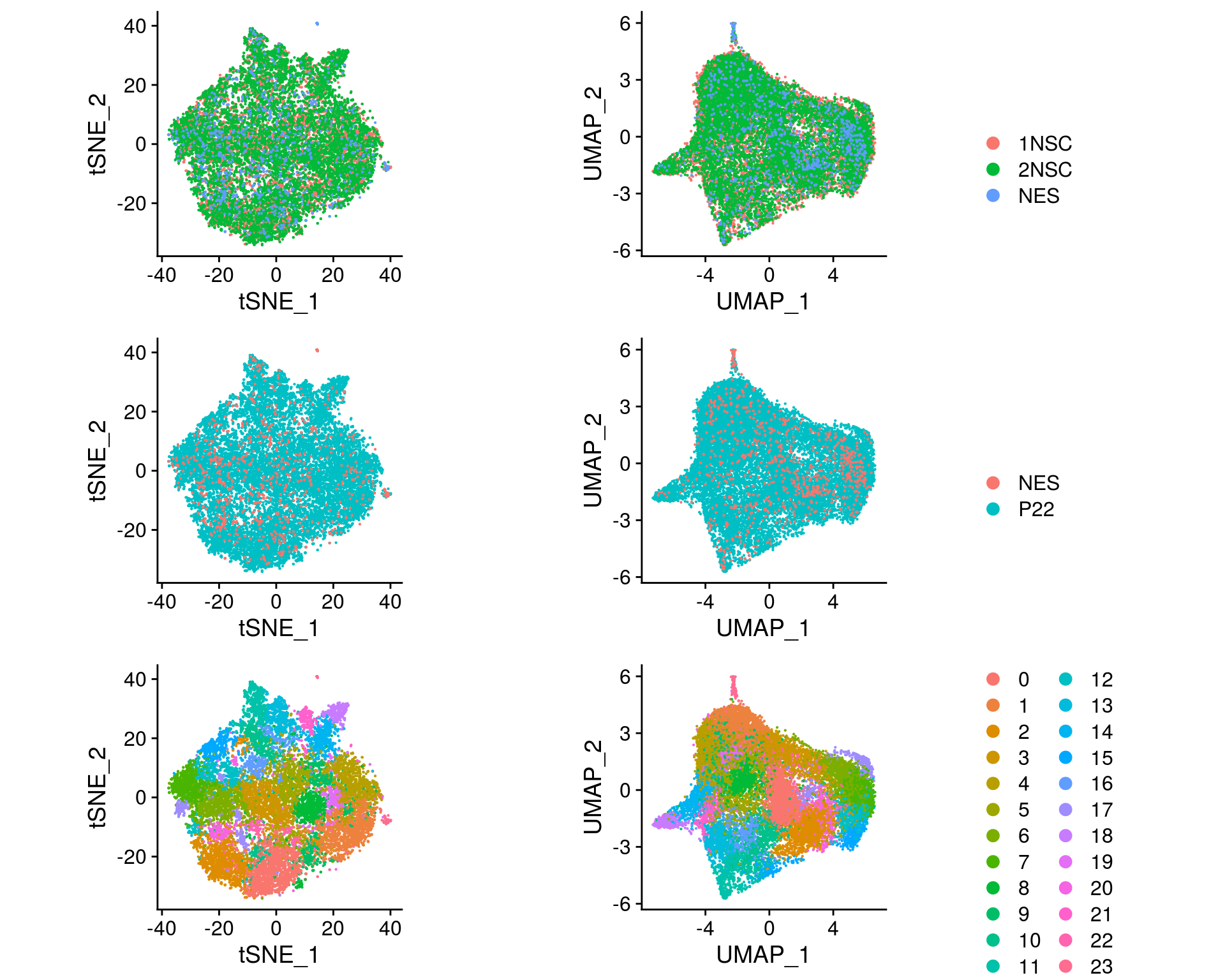
| Version | Author | Date |
|---|---|---|
| a1ebb78 | khembach | 2020-07-08 |
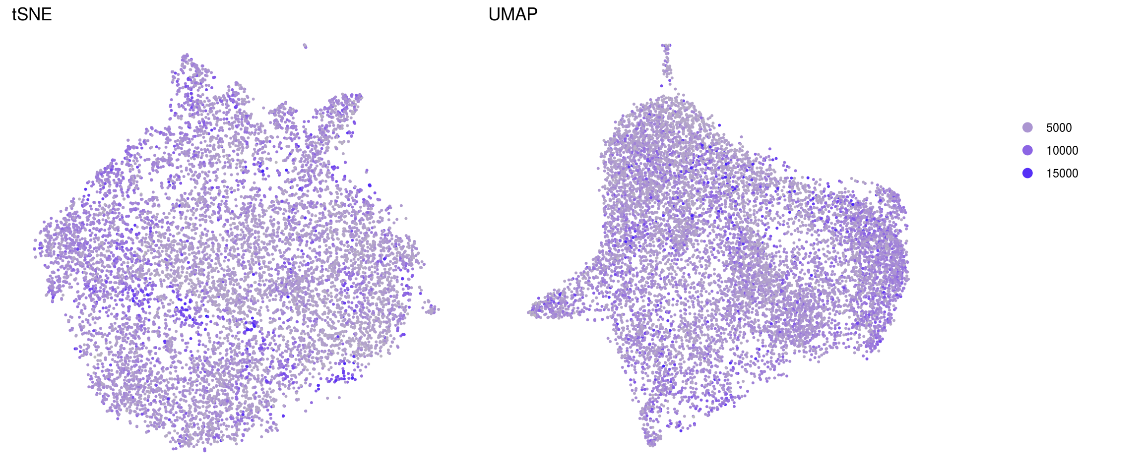
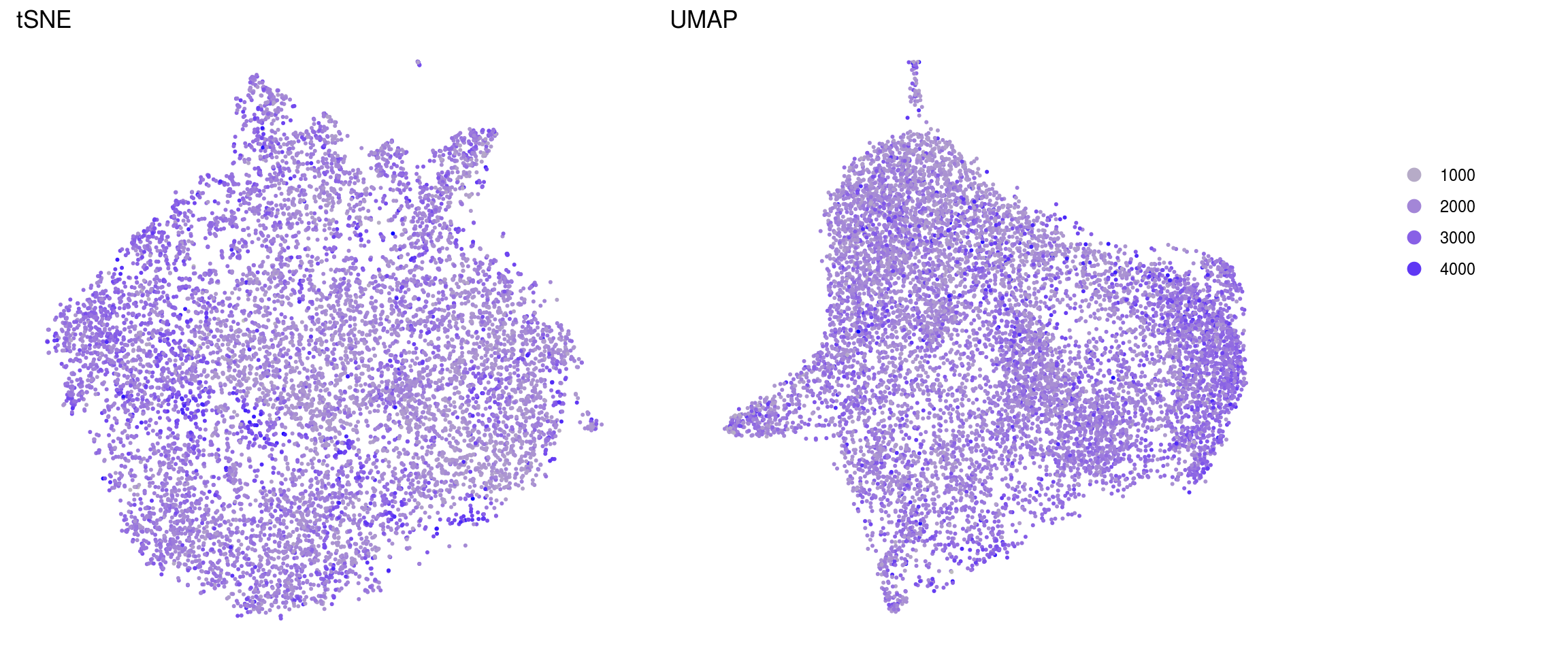
QC on DR plots
cs <- sample(colnames(so), 1e4) ## subsample cells
.plot_features <- function(so, dr, id) {
    FeaturePlot(so, cells = cs, features = id, reduction = dr, pt.size = 0.4,
                cols = c("grey", "blue")) +
        guides(col = guide_legend(nrow = 11,
            override.aes = list(size = 3, alpha = 1))) +
        theme_void() + theme(aspect.ratio = 1)
}
ids <- c("sum", "detected", "subsets_Mt_percent")
for (id in ids) {
    cat("## ", id, "\n")
    p1 <- .plot_features(so, "tsne", id)
    lgd <- get_legend(p1)
    p1 <- p1 + theme(legend.position = "none") + ggtitle("tSNE")
    p2 <- .plot_features(so, "umap", id) + theme(legend.position = "none") +
      ggtitle("UMAP")
    ps <- plot_grid(plotlist = list(p1, p2), nrow = 1)
    p <- plot_grid(ps, lgd, nrow = 1, rel_widths = c(1, 0.2))
    print(p)
    cat("\n\n")
}
Evaluation of cluster before and after integration
We evaluate if cells which were together in a cluster before the integration of the NES cells are still in the same cluster after integration. We use resolution 0.4 for this analysis.
## Load the Seurat object from our NSC analysis
so_before <- readRDS(file.path("output", "NSC_1_clustering.rds"))
so_before <- SetIdent(so_before, value = "integrated_snn_res.0.4")
so_before@meta.data$cluster_id <- Idents(so_before)
table(so_before@meta.data$cluster_id)
   0    1    2    3    4    5    6
5826 3425 3229 2121 1425  665   48
so <- SetIdent(so, value = "integrated_snn_res.0.4")
so@meta.data$cluster_id <- Idents(so)
## subset to our NSCs
cs <- which(so@meta.data$group_id == "P22")
sub <- subset(so, cells = cs)
table(sub@meta.data$cluster_id)
   0    1    2    3    4    5    6
5920 3495 3251 2025 1164  813   71
## join the cluster_ids from both clustering runs
before <- data.frame(cell = colnames(so_before),
cluster_before = so_before@meta.data[,c("cluster_id")])
after <- data.frame(cell = colnames(sub),
cluster_after = sub@meta.data[,c("cluster_id")])
clusters <- before %>% full_join(after)
## check if cells from the same cluster are still in the same cluster
(n_clusters <- table(clusters$cluster_before, clusters$cluster_after))
       0    1    2    3    4    5    6
  0 5360  166   81  109   25   67   18
  1  101 3131   33   20   15  122    3
  2   82   77 3038   27    0    4    1
  3   88   97   89 1827   17    3    0
  4  240   21    8   38 1106   11    1
  5   49    3    2    4    1  606    0
  6    0    0    0    0    0    0   48
fqs <- prop.table(n_clusters, margin = 2)
mat <- as.matrix(unclass(fqs))
Heatmap(mat,
col = rev(brewer.pal(11, "RdGy")[-6]),
name = "Frequency",
cluster_rows = FALSE,
cluster_columns = FALSE,
row_names_side = "left",
row_title = "clusters before NES integration",
column_title = "clusters after NES integration",
column_title_side = "bottom",
rect_gp = gpar(col = "white"),
cell_fun = function(i, j, x, y, width, height, fill)
grid.text(round(mat[j, i] * 100, 2), x = x, y = y,
gp = gpar(col = "white", fontsize = 8)))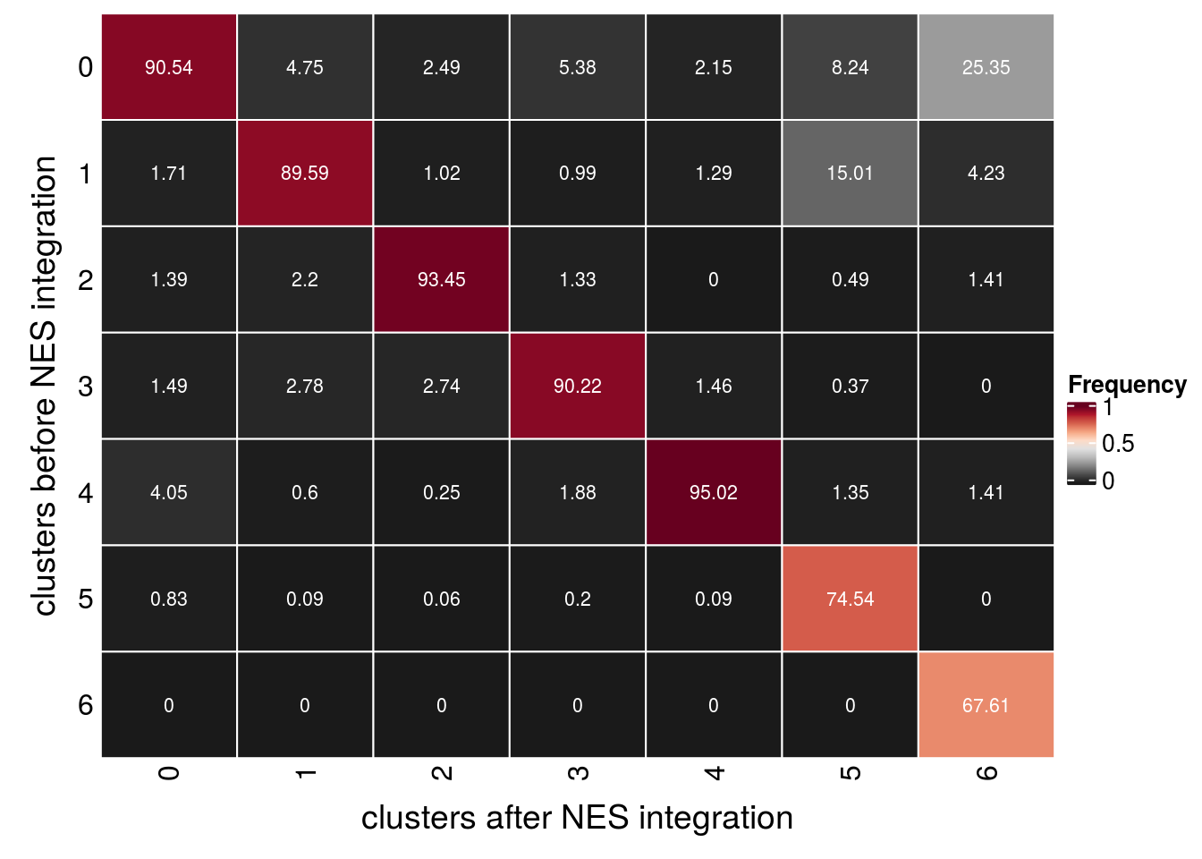
Save Seurat object to RDS
saveRDS(so, file.path("output", "Lam-01-clustering.rds"))
sessionInfo()R version 4.0.0 (2020-04-24)
Platform: x86_64-pc-linux-gnu (64-bit)
Running under: Ubuntu 16.04.6 LTS
Matrix products: default
BLAS: /usr/local/R/R-4.0.0/lib/libRblas.so
LAPACK: /usr/local/R/R-4.0.0/lib/libRlapack.so
locale:
[1] LC_CTYPE=en_US.UTF-8 LC_NUMERIC=C
[3] LC_TIME=en_US.UTF-8 LC_COLLATE=en_US.UTF-8
[5] LC_MONETARY=en_US.UTF-8 LC_MESSAGES=en_US.UTF-8
[7] LC_PAPER=en_US.UTF-8 LC_NAME=C
[9] LC_ADDRESS=C LC_TELEPHONE=C
[11] LC_MEASUREMENT=en_US.UTF-8 LC_IDENTIFICATION=C
attached base packages:
[1] grid parallel stats4 stats graphics grDevices utils
[8] datasets methods base
other attached packages:
[1] HDF5Array_1.16.1 rhdf5_2.32.2
[3] RColorBrewer_1.1-2 ComplexHeatmap_2.4.2
[5] data.table_1.12.8 dplyr_1.0.0
[7] biomaRt_2.44.1 future_1.17.0
[9] rtracklayer_1.48.0 stringr_1.4.0
[11] SingleCellExperiment_1.10.1 SummarizedExperiment_1.18.1
[13] DelayedArray_0.14.0 matrixStats_0.56.0
[15] Biobase_2.48.0 GenomicRanges_1.40.0
[17] GenomeInfoDb_1.24.2 IRanges_2.22.2
[19] S4Vectors_0.26.1 BiocGenerics_0.34.0
[21] Seurat_3.1.5 ggplot2_3.3.2
[23] cowplot_1.0.0 workflowr_1.6.2
loaded via a namespace (and not attached):
[1] circlize_0.4.10 backports_1.1.8 BiocFileCache_1.12.0
[4] plyr_1.8.6 igraph_1.2.5 lazyeval_0.2.2
[7] splines_4.0.0 BiocParallel_1.22.0 listenv_0.8.0
[10] digest_0.6.25 htmltools_0.5.0 magrittr_1.5
[13] memoise_1.1.0 cluster_2.1.0 ROCR_1.0-11
[16] globals_0.12.5 Biostrings_2.56.0 askpass_1.1
[19] prettyunits_1.1.1 colorspace_1.4-1 blob_1.2.1
[22] rappdirs_0.3.1 ggrepel_0.8.2 xfun_0.15
[25] crayon_1.3.4 RCurl_1.98-1.2 jsonlite_1.7.0
[28] survival_3.2-3 zoo_1.8-8 ape_5.4
[31] glue_1.4.1 gtable_0.3.0 zlibbioc_1.34.0
[34] XVector_0.28.0 leiden_0.3.3 GetoptLong_1.0.1
[37] Rhdf5lib_1.10.0 shape_1.4.4 future.apply_1.6.0
[40] scales_1.1.1 DBI_1.1.0 Rcpp_1.0.4.6
[43] viridisLite_0.3.0 progress_1.2.2 clue_0.3-57
[46] reticulate_1.16 bit_1.1-15.2 rsvd_1.0.3
[49] tsne_0.1-3 htmlwidgets_1.5.1 httr_1.4.1
[52] ellipsis_0.3.1 ica_1.0-2 farver_2.0.3
[55] pkgconfig_2.0.3 XML_3.99-0.4 uwot_0.1.8
[58] dbplyr_1.4.4 labeling_0.3 tidyselect_1.1.0
[61] rlang_0.4.6 reshape2_1.4.4 later_1.1.0.1
[64] AnnotationDbi_1.50.1 munsell_0.5.0 tools_4.0.0
[67] generics_0.0.2 RSQLite_2.2.0 ggridges_0.5.2
[70] evaluate_0.14 yaml_2.2.1 knitr_1.29
[73] bit64_0.9-7 fs_1.4.2 fitdistrplus_1.1-1
[76] purrr_0.3.4 RANN_2.6.1 pbapply_1.4-2
[79] nlme_3.1-148 whisker_0.4 compiler_4.0.0
[82] plotly_4.9.2.1 curl_4.3 png_0.1-7
[85] tibble_3.0.1 stringi_1.4.6 RSpectra_0.16-0
[88] lattice_0.20-41 Matrix_1.2-18 vctrs_0.3.1
[91] pillar_1.4.4 lifecycle_0.2.0 lmtest_0.9-37
[94] GlobalOptions_0.1.2 RcppAnnoy_0.0.16 bitops_1.0-6
[97] irlba_2.3.3 httpuv_1.5.4 patchwork_1.0.1
[100] R6_2.4.1 promises_1.1.1 KernSmooth_2.23-17
[103] gridExtra_2.3 codetools_0.2-16 MASS_7.3-51.6
[106] assertthat_0.2.1 openssl_1.4.2 rprojroot_1.3-2
[109] rjson_0.2.20 withr_2.2.0 GenomicAlignments_1.24.0
[112] sctransform_0.2.1 Rsamtools_2.4.0 GenomeInfoDbData_1.2.3
[115] hms_0.5.3 tidyr_1.1.0 rmarkdown_2.3
[118] Rtsne_0.15 git2r_0.27.1