Cell hashing test quality control
Katharina Hembach
5/14/2021
Last updated: 2021-05-17
Checks: 7 0
Knit directory: neural_scRNAseq/
This reproducible R Markdown analysis was created with workflowr (version 1.6.2). The Checks tab describes the reproducibility checks that were applied when the results were created. The Past versions tab lists the development history.
Great! Since the R Markdown file has been committed to the Git repository, you know the exact version of the code that produced these results.
Great job! The global environment was empty. Objects defined in the global environment can affect the analysis in your R Markdown file in unknown ways. For reproduciblity it's best to always run the code in an empty environment.
The command set.seed(20200522) was run prior to running the code in the R Markdown file. Setting a seed ensures that any results that rely on randomness, e.g. subsampling or permutations, are reproducible.
Great job! Recording the operating system, R version, and package versions is critical for reproducibility.
Nice! There were no cached chunks for this analysis, so you can be confident that you successfully produced the results during this run.
Great job! Using relative paths to the files within your workflowr project makes it easier to run your code on other machines.
Great! You are using Git for version control. Tracking code development and connecting the code version to the results is critical for reproducibility.
The results in this page were generated with repository version 7c1517d. See the Past versions tab to see a history of the changes made to the R Markdown and HTML files.
Note that you need to be careful to ensure that all relevant files for the analysis have been committed to Git prior to generating the results (you can use wflow_publish or wflow_git_commit). workflowr only checks the R Markdown file, but you know if there are other scripts or data files that it depends on. Below is the status of the Git repository when the results were generated:
Ignored files:
    Ignored:    .DS_Store
    Ignored:    .Rhistory
    Ignored:    .Rproj.user/
    Ignored:    ._.DS_Store
    Ignored:    ._Filtered.pdf
    Ignored:    ._Rplots.pdf
    Ignored:    ._Unfiltered.pdf
    Ignored:    .__workflowr.yml
    Ignored:    ._coverage.pdf
    Ignored:    ._coverage_sashimi.pdf
    Ignored:    ._coverage_sashimi.png
    Ignored:    ._neural_scRNAseq.Rproj
    Ignored:    ._pbDS_cell_level.pdf
    Ignored:    ._pbDS_top_expr_umap.pdf
    Ignored:    ._pbDS_upset.pdf
    Ignored:    ._sashimi.pdf
    Ignored:    ._stmn2.pdf
    Ignored:    ._tdp.pdf
    Ignored:    analysis/.DS_Store
    Ignored:    analysis/.Rhistory
    Ignored:    analysis/._.DS_Store
    Ignored:    analysis/._01-preprocessing.Rmd
    Ignored:    analysis/._01-preprocessing.html
    Ignored:    analysis/._02.1-SampleQC.Rmd
    Ignored:    analysis/._03-filtering.Rmd
    Ignored:    analysis/._04-clustering.Rmd
    Ignored:    analysis/._04-clustering.knit.md
    Ignored:    analysis/._04.1-cell_cycle.Rmd
    Ignored:    analysis/._05-annotation.Rmd
    Ignored:    analysis/._07-cluster-analysis-all-timepoints.Rmd
    Ignored:    analysis/._Lam-0-NSC_no_integration.Rmd
    Ignored:    analysis/._Lam-01-NSC_integration.Rmd
    Ignored:    analysis/._Lam-02-NSC_annotation.Rmd
    Ignored:    analysis/._NSC-1-clustering.Rmd
    Ignored:    analysis/._NSC-2-annotation.Rmd
    Ignored:    analysis/.__site.yml
    Ignored:    analysis/._additional_filtering.Rmd
    Ignored:    analysis/._additional_filtering_clustering.Rmd
    Ignored:    analysis/._index.Rmd
    Ignored:    analysis/._organoid-01-1-qualtiy-control.Rmd
    Ignored:    analysis/._organoid-01-clustering.Rmd
    Ignored:    analysis/._organoid-02-integration.Rmd
    Ignored:    analysis/._organoid-03-cluster_analysis.Rmd
    Ignored:    analysis/._organoid-04-group_integration.Rmd
    Ignored:    analysis/._organoid-04-stage_integration.Rmd
    Ignored:    analysis/._organoid-05-group_integration_cluster_analysis.Rmd
    Ignored:    analysis/._organoid-05-stage_integration_cluster_analysis.Rmd
    Ignored:    analysis/._organoid-06-1-prepare-sce.Rmd
    Ignored:    analysis/._organoid-06-conos-analysis-Seurat.Rmd
    Ignored:    analysis/._organoid-06-conos-analysis-function.Rmd
    Ignored:    analysis/._organoid-06-conos-analysis.Rmd
    Ignored:    analysis/._organoid-06-group-integration-conos-analysis.Rmd
    Ignored:    analysis/._organoid-07-conos-visualization.Rmd
    Ignored:    analysis/._organoid-07-group-integration-conos-visualization.Rmd
    Ignored:    analysis/._organoid-08-conos-comparison.Rmd
    Ignored:    analysis/._organoid-0x-sample_integration.Rmd
    Ignored:    analysis/01-preprocessing_cache/
    Ignored:    analysis/02-1-SampleQC_cache/
    Ignored:    analysis/02-quality_control_cache/
    Ignored:    analysis/02.1-SampleQC_cache/
    Ignored:    analysis/03-filtering_cache/
    Ignored:    analysis/04-clustering_cache/
    Ignored:    analysis/04.1-cell_cycle_cache/
    Ignored:    analysis/05-annotation_cache/
    Ignored:    analysis/06-clustering-all-timepoints_cache/
    Ignored:    analysis/07-cluster-analysis-all-timepoints_cache/
    Ignored:    analysis/Lam-01-NSC_integration_cache/
    Ignored:    analysis/Lam-02-NSC_annotation_cache/
    Ignored:    analysis/NSC-1-clustering_cache/
    Ignored:    analysis/NSC-2-annotation_cache/
    Ignored:    analysis/TDP-01-preprocessing_cache/
    Ignored:    analysis/TDP-02-quality_control_cache/
    Ignored:    analysis/TDP-03-filtering_cache/
    Ignored:    analysis/TDP-04-clustering_cache/
    Ignored:    analysis/TDP-05-00-filtering-plasmid-QC_cache/
    Ignored:    analysis/TDP-05-plasmid_expression_cache/
    Ignored:    analysis/TDP-06-cluster_analysis_cache/
    Ignored:    analysis/TDP-07-01-STMN2_expression_cache/
    Ignored:    analysis/TDP-07-cluster_12_cache/
    Ignored:    analysis/TDP-08-00-clustering-HA-D96_cache/
    Ignored:    analysis/TDP-08-01-HA-D96-expression-changes_cache/
    Ignored:    analysis/TDP-08-02-TDP_target_genes_cache/
    Ignored:    analysis/TDP-08-clustering-timeline-HA_cache/
    Ignored:    analysis/additional_filtering_cache/
    Ignored:    analysis/additional_filtering_clustering_cache/
    Ignored:    analysis/organoid-01-1-qualtiy-control_cache/
    Ignored:    analysis/organoid-01-clustering_cache/
    Ignored:    analysis/organoid-02-integration_cache/
    Ignored:    analysis/organoid-03-cluster_analysis_cache/
    Ignored:    analysis/organoid-04-group_integration_cache/
    Ignored:    analysis/organoid-04-stage_integration_cache/
    Ignored:    analysis/organoid-05-group_integration_cluster_analysis_cache/
    Ignored:    analysis/organoid-05-stage_integration_cluster_analysis_cache/
    Ignored:    analysis/organoid-06-conos-analysis_cache/
    Ignored:    analysis/organoid-06-conos-analysis_test_cache/
    Ignored:    analysis/organoid-06-group-integration-conos-analysis_cache/
    Ignored:    analysis/organoid-07-conos-visualization_cache/
    Ignored:    analysis/organoid-07-group-integration-conos-visualization_cache/
    Ignored:    analysis/organoid-08-conos-comparison_cache/
    Ignored:    analysis/organoid-0x-sample_integration_cache/
    Ignored:    analysis/sample5_QC_cache/
    Ignored:    analysis/timepoints-01-organoid-integration_cache/
    Ignored:    analysis/timepoints-02-cluster-analysis_cache/
    Ignored:    data/.DS_Store
    Ignored:    data/._.DS_Store
    Ignored:    data/._.smbdeleteAAA17ed8b4b
    Ignored:    data/._Lam_figure2_markers.R
    Ignored:    data/._README.md
    Ignored:    data/._Reactive_astrocytes_markers.xlsx
    Ignored:    data/._known_NSC_markers.R
    Ignored:    data/._known_cell_type_markers.R
    Ignored:    data/._metadata.csv
    Ignored:    data/._virus_cell_tropism_markers.R
    Ignored:    data/._~$Reactive_astrocytes_markers.xlsx
    Ignored:    data/data_sushi/
    Ignored:    data/filtered_feature_matrices/
    Ignored:    output/.DS_Store
    Ignored:    output/._.DS_Store
    Ignored:    output/._NSC_cluster2_marker_genes.txt
    Ignored:    output/._TDP-06-no_integration_cluster12_marker_genes.txt
    Ignored:    output/._TDP-06-no_integration_cluster13_marker_genes.txt
    Ignored:    output/._organoid_integration_cluster1_marker_genes.txt
    Ignored:    output/._tbl_TDP-08-01-muscat_cluster_0.txt
    Ignored:    output/._tbl_TDP-08-01-muscat_cluster_1.txt
    Ignored:    output/._tbl_TDP-08-01-muscat_cluster_10.txt
    Ignored:    output/._tbl_TDP-08-01-muscat_cluster_11.txt
    Ignored:    output/._tbl_TDP-08-01-muscat_cluster_12.txt
    Ignored:    output/._tbl_TDP-08-01-muscat_cluster_13.txt
    Ignored:    output/._tbl_TDP-08-01-muscat_cluster_14.txt
    Ignored:    output/._tbl_TDP-08-01-muscat_cluster_5.txt
    Ignored:    output/._tbl_TDP-08-01-muscat_cluster_7.txt
    Ignored:    output/._tbl_TDP-08-01-muscat_cluster_8.txt
    Ignored:    output/._tbl_TDP-08-01-muscat_cluster_all.xlsx
    Ignored:    output/._tbl_TDP-08-02-targets_hek_cluster_0.txt
    Ignored:    output/._tbl_TDP-08-02-targets_hek_cluster_1.txt
    Ignored:    output/._tbl_TDP-08-02-targets_hek_cluster_10.txt
    Ignored:    output/._tbl_TDP-08-02-targets_hek_cluster_11.txt
    Ignored:    output/._tbl_TDP-08-02-targets_hek_cluster_12.txt
    Ignored:    output/._tbl_TDP-08-02-targets_hek_cluster_13.txt
    Ignored:    output/._tbl_TDP-08-02-targets_hek_cluster_14.txt
    Ignored:    output/._tbl_TDP-08-02-targets_hek_cluster_5.txt
    Ignored:    output/._tbl_TDP-08-02-targets_hek_cluster_7.txt
    Ignored:    output/._tbl_TDP-08-02-targets_hek_cluster_8.txt
    Ignored:    output/._tbl_TDP-08-02-targets_hek_cluster_all.xlsx
    Ignored:    output/._~$tbl_TDP-08-02-targets_hek_cluster_all.xlsx
    Ignored:    output/CH-test-01-preprocessing.rds
    Ignored:    output/Lam-01-clustering.rds
    Ignored:    output/NSC_1_clustering.rds
    Ignored:    output/NSC_cluster1_marker_genes.txt
    Ignored:    output/NSC_cluster2_marker_genes.txt
    Ignored:    output/NSC_cluster3_marker_genes.txt
    Ignored:    output/NSC_cluster4_marker_genes.txt
    Ignored:    output/NSC_cluster5_marker_genes.txt
    Ignored:    output/NSC_cluster6_marker_genes.txt
    Ignored:    output/NSC_cluster7_marker_genes.txt
    Ignored:    output/TDP-06-no_integration_cluster0_marker_genes.txt
    Ignored:    output/TDP-06-no_integration_cluster10_marker_genes.txt
    Ignored:    output/TDP-06-no_integration_cluster11_marker_genes.txt
    Ignored:    output/TDP-06-no_integration_cluster12_marker_genes.txt
    Ignored:    output/TDP-06-no_integration_cluster13_marker_genes.txt
    Ignored:    output/TDP-06-no_integration_cluster14_marker_genes.txt
    Ignored:    output/TDP-06-no_integration_cluster15_marker_genes.txt
    Ignored:    output/TDP-06-no_integration_cluster16_marker_genes.txt
    Ignored:    output/TDP-06-no_integration_cluster17_marker_genes.txt
    Ignored:    output/TDP-06-no_integration_cluster1_marker_genes.txt
    Ignored:    output/TDP-06-no_integration_cluster2_marker_genes.txt
    Ignored:    output/TDP-06-no_integration_cluster3_marker_genes.txt
    Ignored:    output/TDP-06-no_integration_cluster4_marker_genes.txt
    Ignored:    output/TDP-06-no_integration_cluster5_marker_genes.txt
    Ignored:    output/TDP-06-no_integration_cluster6_marker_genes.txt
    Ignored:    output/TDP-06-no_integration_cluster7_marker_genes.txt
    Ignored:    output/TDP-06-no_integration_cluster8_marker_genes.txt
    Ignored:    output/TDP-06-no_integration_cluster9_marker_genes.txt
    Ignored:    output/TDP-06_scran_markers.rds
    Ignored:    output/additional_filtering.rds
    Ignored:    output/conos/
    Ignored:    output/conos_organoid-06-conos-analysis.rds
    Ignored:    output/conos_organoid-06-group-integration-conos-analysis.rds
    Ignored:    output/figures/
    Ignored:    output/organoid_integration_cluster10_marker_genes.txt
    Ignored:    output/organoid_integration_cluster11_marker_genes.txt
    Ignored:    output/organoid_integration_cluster12_marker_genes.txt
    Ignored:    output/organoid_integration_cluster13_marker_genes.txt
    Ignored:    output/organoid_integration_cluster14_marker_genes.txt
    Ignored:    output/organoid_integration_cluster15_marker_genes.txt
    Ignored:    output/organoid_integration_cluster16_marker_genes.txt
    Ignored:    output/organoid_integration_cluster17_marker_genes.txt
    Ignored:    output/organoid_integration_cluster1_marker_genes.txt
    Ignored:    output/organoid_integration_cluster2_marker_genes.txt
    Ignored:    output/organoid_integration_cluster3_marker_genes.txt
    Ignored:    output/organoid_integration_cluster4_marker_genes.txt
    Ignored:    output/organoid_integration_cluster5_marker_genes.txt
    Ignored:    output/organoid_integration_cluster6_marker_genes.txt
    Ignored:    output/organoid_integration_cluster7_marker_genes.txt
    Ignored:    output/organoid_integration_cluster8_marker_genes.txt
    Ignored:    output/organoid_integration_cluster9_marker_genes.txt
    Ignored:    output/res_TDP-08-01-muscat.rds
    Ignored:    output/sce_01_preprocessing.rds
    Ignored:    output/sce_02_quality_control.rds
    Ignored:    output/sce_03_filtering.rds
    Ignored:    output/sce_03_filtering_all_genes.rds
    Ignored:    output/sce_06-1-prepare-sce.rds
    Ignored:    output/sce_TDP-08-01-muscat.rds
    Ignored:    output/sce_TDP_01_preprocessing.rds
    Ignored:    output/sce_TDP_02_quality_control.rds
    Ignored:    output/sce_TDP_03_filtering.rds
    Ignored:    output/sce_TDP_03_filtering_all_genes.rds
    Ignored:    output/sce_organoid-01-clustering.rds
    Ignored:    output/sce_preprocessing.rds
    Ignored:    output/so_04-stage_integration.rds
    Ignored:    output/so_04_1_cell_cycle.rds
    Ignored:    output/so_04_clustering.rds
    Ignored:    output/so_06-clustering_all_timepoints.rds
    Ignored:    output/so_08-00_clustering_HA_D96.rds
    Ignored:    output/so_08-clustering_timeline_HA.rds
    Ignored:    output/so_0x-sample_integration.rds
    Ignored:    output/so_TDP-06-cluster-analysis.rds
    Ignored:    output/so_TDP_04_clustering.rds
    Ignored:    output/so_TDP_05_plasmid_expression.rds
    Ignored:    output/so_additional_filtering_clustering.rds
    Ignored:    output/so_integrated_organoid-02-integration.rds
    Ignored:    output/so_merged_organoid-02-integration.rds
    Ignored:    output/so_organoid-01-clustering.rds
    Ignored:    output/so_sample_organoid-01-clustering.rds
    Ignored:    output/so_timepoints-01-organoid_integration.rds
    Ignored:    output/tbl_TDP-08-01-muscat.rds
    Ignored:    output/tbl_TDP-08-01-muscat_cluster_0.txt
    Ignored:    output/tbl_TDP-08-01-muscat_cluster_1.txt
    Ignored:    output/tbl_TDP-08-01-muscat_cluster_10.txt
    Ignored:    output/tbl_TDP-08-01-muscat_cluster_11.txt
    Ignored:    output/tbl_TDP-08-01-muscat_cluster_12.txt
    Ignored:    output/tbl_TDP-08-01-muscat_cluster_13.txt
    Ignored:    output/tbl_TDP-08-01-muscat_cluster_14.txt
    Ignored:    output/tbl_TDP-08-01-muscat_cluster_5.txt
    Ignored:    output/tbl_TDP-08-01-muscat_cluster_7.txt
    Ignored:    output/tbl_TDP-08-01-muscat_cluster_8.txt
    Ignored:    output/tbl_TDP-08-01-muscat_cluster_all.xlsx
    Ignored:    output/tbl_TDP-08-02-targets_hek.rds
    Ignored:    output/tbl_TDP-08-02-targets_hek_cluster_0.txt
    Ignored:    output/tbl_TDP-08-02-targets_hek_cluster_1.txt
    Ignored:    output/tbl_TDP-08-02-targets_hek_cluster_10.txt
    Ignored:    output/tbl_TDP-08-02-targets_hek_cluster_11.txt
    Ignored:    output/tbl_TDP-08-02-targets_hek_cluster_12.txt
    Ignored:    output/tbl_TDP-08-02-targets_hek_cluster_13.txt
    Ignored:    output/tbl_TDP-08-02-targets_hek_cluster_14.txt
    Ignored:    output/tbl_TDP-08-02-targets_hek_cluster_5.txt
    Ignored:    output/tbl_TDP-08-02-targets_hek_cluster_7.txt
    Ignored:    output/tbl_TDP-08-02-targets_hek_cluster_8.txt
    Ignored:    output/tbl_TDP-08-02-targets_hek_cluster_all.xlsx
    Ignored:    output/~$tbl_TDP-08-02-targets_hek_cluster_all.xlsx
    Ignored:    scripts/.DS_Store
    Ignored:    scripts/._.DS_Store
    Ignored:    scripts/._bu_Rcode.R
    Ignored:    scripts/._plasmid_expression.sh
    Ignored:    scripts/._plasmid_expression_cell_hashing_test.sh
    Ignored:    scripts/._prepare_salmon_transcripts.R
    Ignored:    scripts/._prepare_salmon_transcripts_cell_hashing_test.R

Untracked files:
    Untracked:  Filtered.pdf
    Untracked:  Rplots.pdf
    Untracked:  Unfiltered
    Untracked:  Unfiltered.pdf
    Untracked:  analysis/Lam-0-NSC_no_integration.Rmd
    Untracked:  analysis/TDP-07-01-STMN2_expression copy.Rmd
    Untracked:  analysis/additional_filtering.Rmd
    Untracked:  analysis/additional_filtering_clustering.Rmd
    Untracked:  analysis/organoid-01-1-qualtiy-control.Rmd
    Untracked:  analysis/organoid-06-conos-analysis-Seurat.Rmd
    Untracked:  analysis/organoid-06-conos-analysis-function.Rmd
    Untracked:  analysis/organoid-07-conos-visualization.Rmd
    Untracked:  analysis/organoid-07-group-integration-conos-visualization.Rmd
    Untracked:  analysis/organoid-08-conos-comparison.Rmd
    Untracked:  analysis/organoid-0x-sample_integration.Rmd
    Untracked:  analysis/sample5_QC.Rmd
    Untracked:  coverage.pdf
    Untracked:  coverage_sashimi.pdf
    Untracked:  coverage_sashimi.png
    Untracked:  data/Homo_sapiens.GRCh38.98.sorted.gtf
    Untracked:  data/Kanton_et_al/
    Untracked:  data/Lam_et_al/
    Untracked:  data/Sep2020/
    Untracked:  data/cell_hashing_test/
    Untracked:  data/reference/
    Untracked:  data/virus_cell_tropism_markers.R
    Untracked:  data/~$Reactive_astrocytes_markers.xlsx
    Untracked:  pbDS_cell_level.pdf
    Untracked:  pbDS_heatmap.pdf
    Untracked:  pbDS_top_expr_umap.pdf
    Untracked:  pbDS_upset.pdf
    Untracked:  sashimi.pdf
    Untracked:  scripts/bu_Rcode.R
    Untracked:  scripts/bu_code.Rmd
    Untracked:  scripts/plasmid_expression_cell_hashing_test.sh
    Untracked:  scripts/prepare_salmon_transcripts_cell_hashing_test.R
    Untracked:  scripts/salmon-latest_linux_x86_64/
    Untracked:  stmn2.pdf
    Untracked:  tdp.pdf

Unstaged changes:
    Modified:   analysis/05-annotation.Rmd
    Modified:   analysis/TDP-04-clustering.Rmd
    Modified:   analysis/TDP-08-01-HA-D96-expression-changes.Rmd
    Modified:   analysis/_site.yml
    Modified:   analysis/organoid-02-integration.Rmd
    Modified:   analysis/organoid-04-group_integration.Rmd
    Modified:   analysis/organoid-06-conos-analysis.Rmd
Note that any generated files, e.g. HTML, png, CSS, etc., are not included in this status report because it is ok for generated content to have uncommitted changes.
These are the previous versions of the repository in which changes were made to the R Markdown (analysis/CH-test-01-preprocessing.Rmd) and HTML (docs/CH-test-01-preprocessing.html) files. If you've configured a remote Git repository (see ?wflow_git_remote), click on the hyperlinks in the table below to view the files as they were in that past version.
| File | Version | Author | Date | Message |
|---|---|---|---|---|
| Rmd | 7c1517d | khembach | 2021-05-17 | run HTO demultipxing before and after filtering of low quality cells |
| html | 4f37f3d | khembach | 2021-05-14 | Build site. |
| Rmd | d03901f | khembach | 2021-05-14 | preprocessing and quality control of HTO test experiment |
Load packages
library(DropletUtils)
library(BiocParallel)
library(ggplot2)
library(scater)
library(readxl)
library(Seurat)
library(scales)
library(viridis)
library(dplyr)
Importing CellRanger output and metadata
fs <- file.path("data", "cell_hashing_test",
                "CellRangerCount_57443_2021-05-12--11-37-28", "HashTag_test",
                "filtered_feature_bc_matrix.h5")
names(fs) <- "cell_hashing_test"
sce_raw <- read10xCounts(samples = fs)

# rename colnames and dimnames
rowData(sce_raw)$Type <- NULL
names(rowData(sce_raw)) <- c("ensembl_id", "symbol")
names(colData(sce_raw)) <- c("sample_id", "barcode")
sce_raw$sample_id <- factor(sce_raw$sample_id)

# load metadata
meta <- read_excel(file.path("data", "cell_hashing_test", "SampleName_feature_ref_MHP.xlsm"))
m <- match(meta$name, rowData(sce_raw)$symbol)

## separate gene counts from HTO counts
rowData(sce_raw) %>% tail
DataFrame with 6 rows and 2 columns
ensembl_id symbol
<character> <character>
ENSG00000276017 ENSG00000276017 AC007325.1
ENSG00000278817 ENSG00000278817 AC007325.4
ENSG00000277196 ENSG00000277196 AC007325.2
B0253 B0253 Hashtag3
B0254 B0254 Hashtag4
B0257 B0257 Hashtag7sce <- sce_raw[-m,]
dimnames(sce) <- list(with(rowData(sce), paste(ensembl_id, symbol, sep = ".")),
with(colData(sce), paste(barcode, sample_id, sep = ".")))Quality control
We compute cell-level QC.
# remove empty rows
sce <- sce[rowSums(counts(sce) > 0) > 0, ]
dim(sce)
[1] 18824 17631(mito <- grep("MT-", rownames(sce), value = TRUE)) [1] "ENSG00000210049.MT-TF" "ENSG00000211459.MT-RNR1"
[3] "ENSG00000210077.MT-TV" "ENSG00000210082.MT-RNR2"
[5] "ENSG00000209082.MT-TL1" "ENSG00000198888.MT-ND1"
[7] "ENSG00000210100.MT-TI" "ENSG00000210107.MT-TQ"
[9] "ENSG00000210112.MT-TM" "ENSG00000198763.MT-ND2"
[11] "ENSG00000210117.MT-TW" "ENSG00000210127.MT-TA"
[13] "ENSG00000210135.MT-TN" "ENSG00000210140.MT-TC"
[15] "ENSG00000210144.MT-TY" "ENSG00000198804.MT-CO1"
[17] "ENSG00000210151.MT-TS1" "ENSG00000210154.MT-TD"
[19] "ENSG00000198712.MT-CO2" "ENSG00000210156.MT-TK"
[21] "ENSG00000228253.MT-ATP8" "ENSG00000198899.MT-ATP6"
[23] "ENSG00000198938.MT-CO3" "ENSG00000210164.MT-TG"
[25] "ENSG00000198840.MT-ND3" "ENSG00000210174.MT-TR"
[27] "ENSG00000212907.MT-ND4L" "ENSG00000198886.MT-ND4"
[29] "ENSG00000210176.MT-TH" "ENSG00000210184.MT-TS2"
[31] "ENSG00000210191.MT-TL2" "ENSG00000198786.MT-ND5"
[33] "ENSG00000198695.MT-ND6" "ENSG00000210194.MT-TE"
[35] "ENSG00000198727.MT-CYB" "ENSG00000210195.MT-TT"
[37] "ENSG00000210196.MT-TP" sce <- addPerCellQC(sce, subsets = list(Mt = mito))
# we compute the fraction of mitochondrial genes and the logit of it
sce$subsets_Mt_fraction <- (sce$subsets_Mt_percent + 0.001) /100
sce$subsets_Mt_fraction_logit <- qlogis(sce$subsets_Mt_fraction + 0.001)
# library size
summary(sce$sum) Min. 1st Qu. Median Mean 3rd Qu. Max.
500 642 862 5216 5818 96619 # number of detected genes per cell
summary(sce$detected) Min. 1st Qu. Median Mean 3rd Qu. Max.
302 491 609 1650 2540 9081 # percentage of counts that come from mitochondrial genes:
summary(sce$subsets_Mt_percent) Min. 1st Qu. Median Mean 3rd Qu. Max.
0.01666 3.86824 7.70896 9.93049 13.29026 87.60776 Diagnostic plots
The number of counts per cell:
plotColData(sce, x = "sample_id", y = "sum") + scale_y_log10()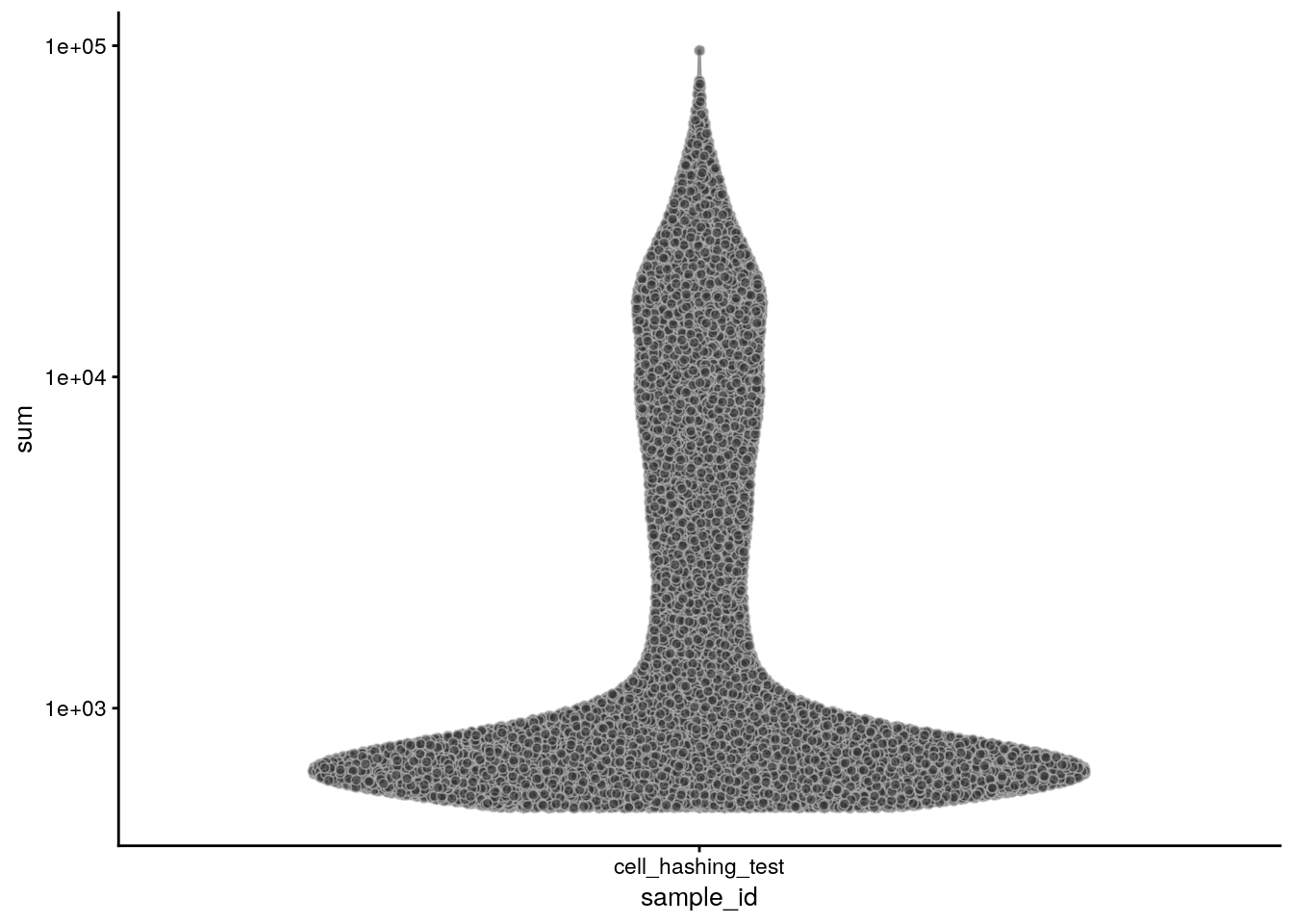
| Version | Author | Date |
|---|---|---|
| 4f37f3d | khembach | 2021-05-14 |
The number of genes:
plotColData(sce, x = "sample_id", y = "detected") + scale_y_log10() 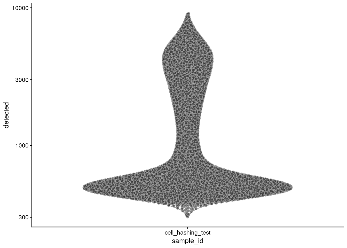
| Version | Author | Date |
|---|---|---|
| 4f37f3d | khembach | 2021-05-14 |
The percentage of mitochondrial genes:
plotColData(sce, x = "sample_id", y = "subsets_Mt_percent")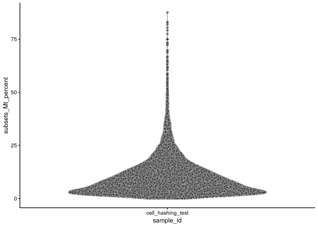
| Version | Author | Date |
|---|---|---|
| 4f37f3d | khembach | 2021-05-14 |
We plot the total number of counts against the number of detected genes and color by the fraction of mitochondrial genes:
cd <- data.frame(colData(sce))
ggplot(cd, aes(x = sum, y = detected, color = subsets_Mt_fraction)) +
  geom_point(alpha = 0.7) +
  geom_density_2d(color = "grey", bins = 6) +
  scale_x_log10() +
  scale_y_log10() +
  facet_wrap(~sample_id) +
  theme_bw() +
  theme(axis.text.x = element_text(angle = 45, hjust = 1)) +
  xlab("sum of counts") +
  ylab("number of detected genes") +
  labs(color = "mitochondrial fraction") +
  scale_color_viridis(trans = "logit", breaks = c(0.01, 0.1, 0.25, 0.5, 0.75))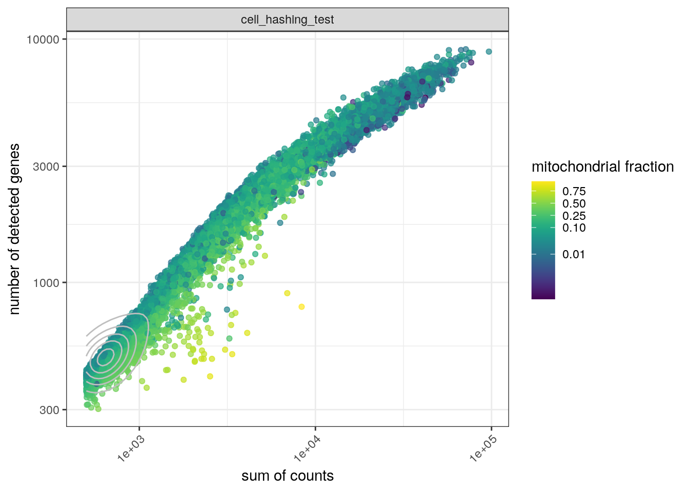
| Version | Author | Date |
|---|---|---|
| 4f37f3d | khembach | 2021-05-14 |
We plot the total number of counts against the mitochondrial content. Well-behaved cells should have many expressed genes and a low fraction of mitochondrial genes. High mitochondrial content indicates empty or damaged cells.
ggplot(cd, aes(x = sum, y = subsets_Mt_fraction)) +
  geom_point(color = "darkgrey", alpha = 0.3) +
  geom_density_2d(color = "lightblue") +
  scale_x_log10() +
  scale_y_continuous(trans = 'logit',
                     breaks = c(0.01, 0.05, 0.1, 0.2, 0.5, 0.75)) +
  facet_wrap(~sample_id) +
  theme_bw() +
  theme(axis.text.x = element_text(angle = 45, hjust = 1)) +
  xlab("sum of counts") +
  ylab("logit(mitochondrial fraction)")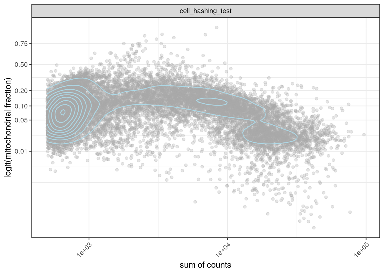
| Version | Author | Date |
|---|---|---|
| 4f37f3d | khembach | 2021-05-14 |
Create Seurat object and split gene and HTO counts
## convert DDelayedMatrix to dgCMatrix for import into Seurat object
counts <- as(counts(sce, withDimnames = FALSE), "dgCMatrix")
colnames(counts) <- colnames(counts(sce))
rownames(counts) <- rownames(counts(sce))

so <- CreateSeuratObject(
    counts = counts,
    meta.data = data.frame(colData(sce)),
    project = "cell_hashing_test")
Warning: Feature names cannot have underscores ('_'), replacing with dashes
('-')## add HTO data as independent assay
hto_counts <- as(counts(sce_raw, withDimnames = FALSE)[m,with(colData(sce),
paste(barcode, sample_id, sep = ".")) %in%
colnames(sce)], "dgCMatrix")
colnames(hto_counts) <- colnames(sce)
rownames(hto_counts) <- rownames(sce_raw)[m]
so[["HTO"]] <- CreateAssayObject(counts = hto_counts)Data normalization
DefaultAssay(so) <- "RNA"
# Normalize RNA data with log normalization
so <- NormalizeData(so)
# Find and scale variable features
so <- FindVariableFeatures(so, selection.method = "mean.var.plot")
so <- ScaleData(so, features = VariableFeatures(so))

# Normalize HTO data, here we use centered log-ratio (CLR) transformation
so <- NormalizeData(so, assay = "HTO", normalization.method = "CLR")
Demultiplex cells based on HTO enrichment
so <- HTODemux(so, assay = "HTO", positive.quantile = 0.99)Cutoff for B0253 : 312 readsCutoff for B0254 : 446 readsCutoff for B0257 : 369 readsVisualize results
# Global classification results
table(so$HTO_classification.global)
 Doublet Negative  Singlet
    2861    10318     4452
# Group cells based on the max HTO signal
Idents(so) <- "HTO_maxID"
# Group cells based on the max HTO signal
RidgePlot(so, assay = "HTO", features = rownames(so[["HTO"]]), ncol = 3)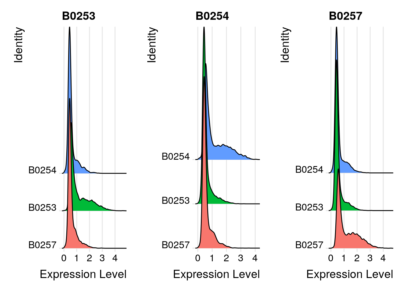
| Version | Author | Date |
|---|---|---|
| 4f37f3d | khembach | 2021-05-14 |
# Visualize pairs of HTO signals to check mutual exclusivity in singlets
DefaultAssay(object = so) <- "HTO"
FeatureScatter(so, feature1 = "B0253", feature2 = "B0254")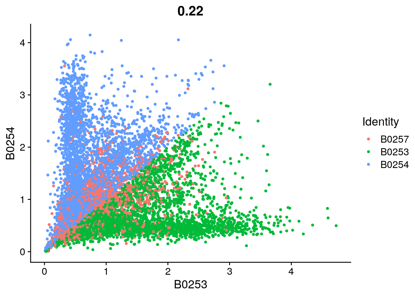
| Version | Author | Date |
|---|---|---|
| 4f37f3d | khembach | 2021-05-14 |
FeatureScatter(so, feature1 = "B0257", feature2 = "B0254")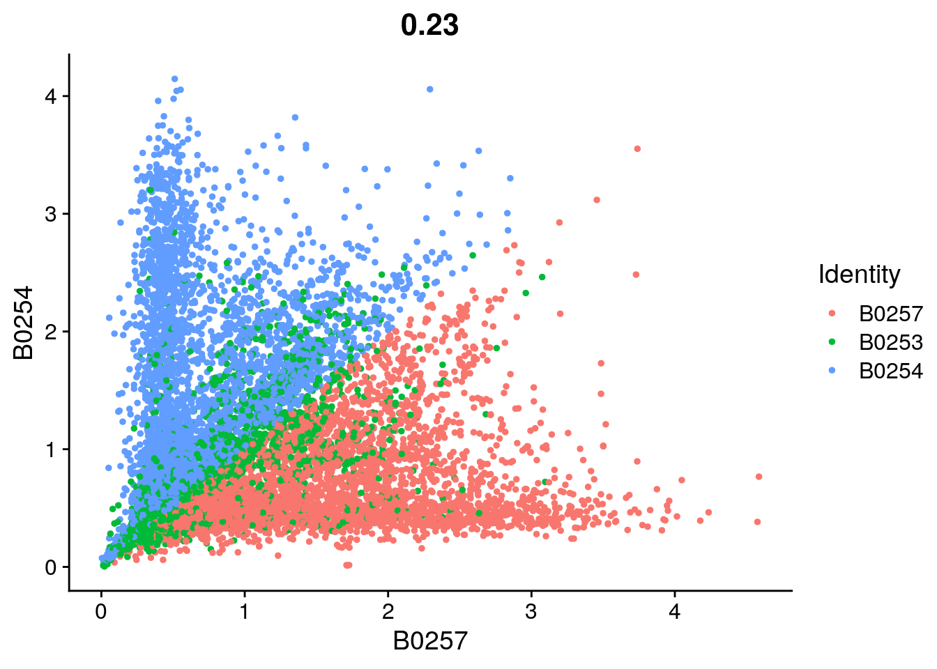
| Version | Author | Date |
|---|---|---|
| 4f37f3d | khembach | 2021-05-14 |
FeatureScatter(so, feature1 = "B0253", feature2 = "B0257")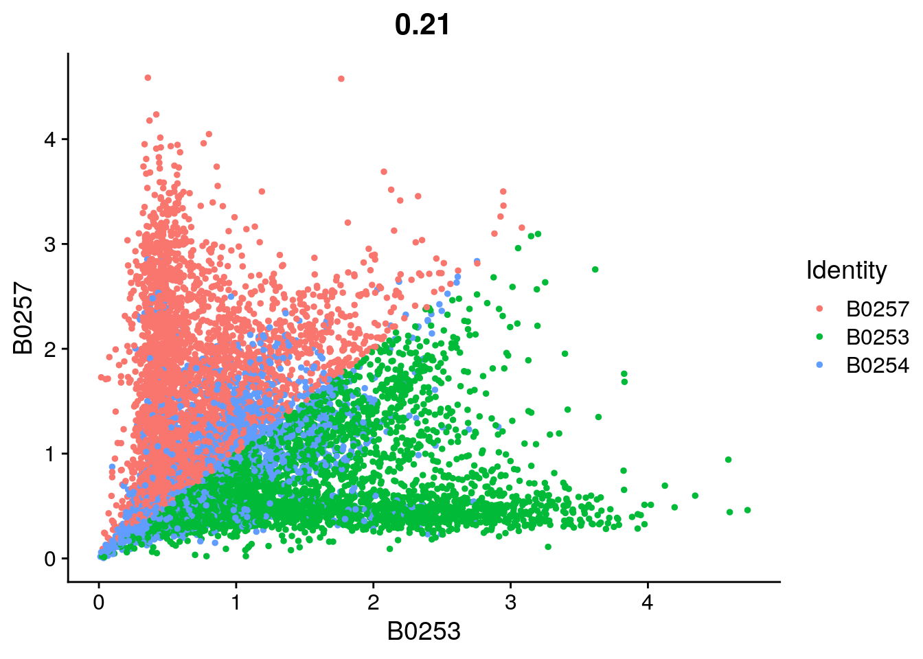
| Version | Author | Date |
|---|---|---|
| 4f37f3d | khembach | 2021-05-14 |
## compare number of UMIs for singlet's, doublets and negative cells
Idents(so) <- "HTO_classification.global"
VlnPlot(so, features = "nCount_HTO", pt.size = 0.1, log = TRUE)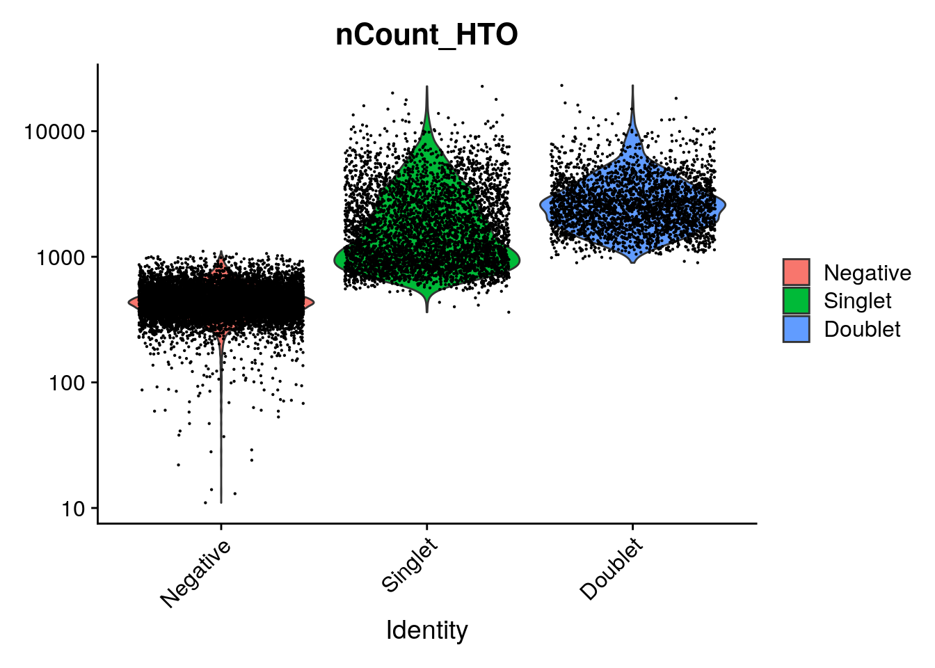
| Version | Author | Date |
|---|---|---|
| 4f37f3d | khembach | 2021-05-14 |
VlnPlot(so, features = "nCount_RNA", pt.size = 0.1, log = TRUE)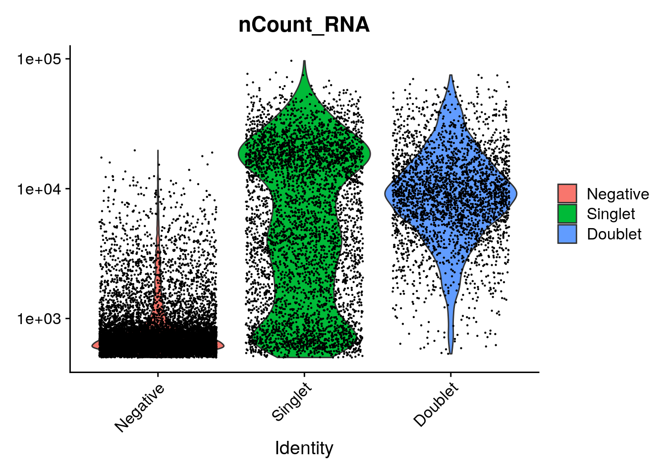
| Version | Author | Date |
|---|---|---|
| 4f37f3d | khembach | 2021-05-14 |
## tSNE for HTOs
# First, we will remove negative cells from the object
subs <- subset(so, idents = "Negative", invert = TRUE)
subs$HTO_classification %>% table
.
B0253 B0253_B0254 B0253_B0257 B0254 B0254_B0257 B0257
1424 916 875 1329 1070 1699 # Calculate a tSNE embedding of the HTO data
DefaultAssay(subs) <- "HTO"
subs <- ScaleData(subs, features = rownames(subs),
verbose = FALSE)
subs <- RunPCA(subs, features = rownames(subs), approx = FALSE, npcs = 3)Warning in print.DimReduc(x = reduction.data, dims = ndims.print, nfeatures =
nfeatures.print): Only 3 dimensions have been computed.Warning: Requested number is larger than the number of available items (3).
Setting to 3.
Warning: Requested number is larger than the number of available items (3).
Setting to 3.
Warning: Requested number is larger than the number of available items (3).
Setting to 3.subs <- RunTSNE(subs, dims = 1:3, perplexity = 100)
Idents(subs) <- "HTO_classification.global"
DimPlot(subs)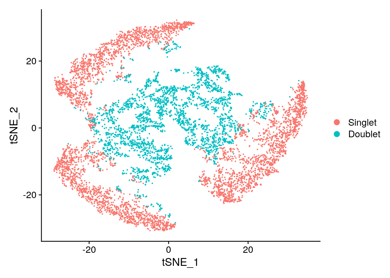
| Version | Author | Date |
|---|---|---|
| 4f37f3d | khembach | 2021-05-14 |
Idents(subs) <- 'HTO_classification'
DimPlot(subs)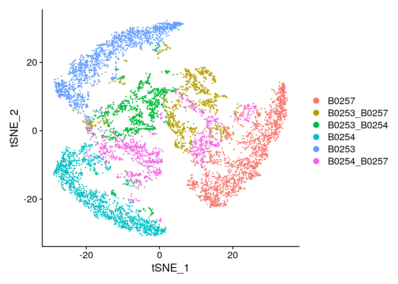
| Version | Author | Date |
|---|---|---|
| 4f37f3d | khembach | 2021-05-14 |
# HTO heatmap
HTOHeatmap(so, assay = "HTO", ncells = 5000)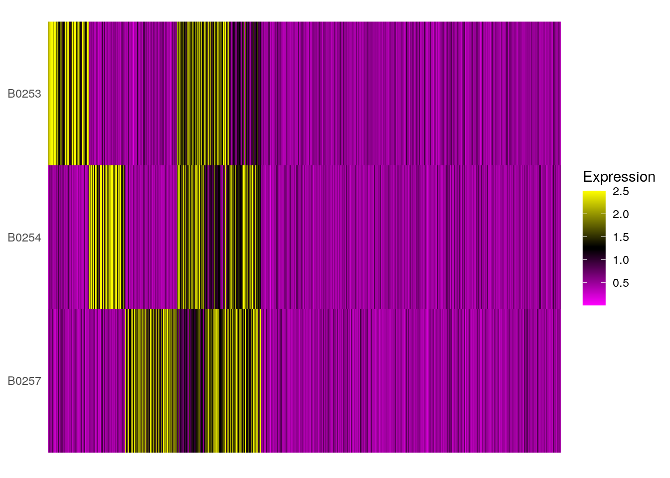
| Version | Author | Date |
|---|---|---|
| 4f37f3d | khembach | 2021-05-14 |
Cluster based on gene counts and visualize cells
DefaultAssay(so) <- "RNA"
# Extract the singlets
singlets <- subset(so, idents = "Singlet")
singlets$HTO_classification %>% table
.
B0253 B0254 B0257
1424 1329 1699 # Select the top 1000 most variable features
singlets <- FindVariableFeatures(singlets, selection.method = "mean.var.plot")
# Scaling RNA data, we only scale the variable features here for efficiency
singlets <- ScaleData(singlets, features = VariableFeatures(singlets))
# Run PCA
singlets <- RunPCA(singlets, features = VariableFeatures(singlets))
# We select the top 10 PCs for clustering and tSNE based on PCElbowPlot
singlets <- FindNeighbors(singlets, reduction = "pca", dims = 1:10)
singlets <- FindClusters(singlets, resolution = 0.6, verbose = FALSE)
singlets <- RunTSNE(singlets, reduction = "pca", dims = 1:10)
singlets <- RunUMAP(singlets, reduction = "pca", dims = 1:10)Warning: The default method for RunUMAP has changed from calling Python UMAP via reticulate to the R-native UWOT using the cosine metric
To use Python UMAP via reticulate, set umap.method to 'umap-learn' and metric to 'correlation'
This message will be shown once per session# Projecting singlet identities on TSNE visualization
DimPlot(singlets, group.by = "HTO_classification", reduction = "tsne")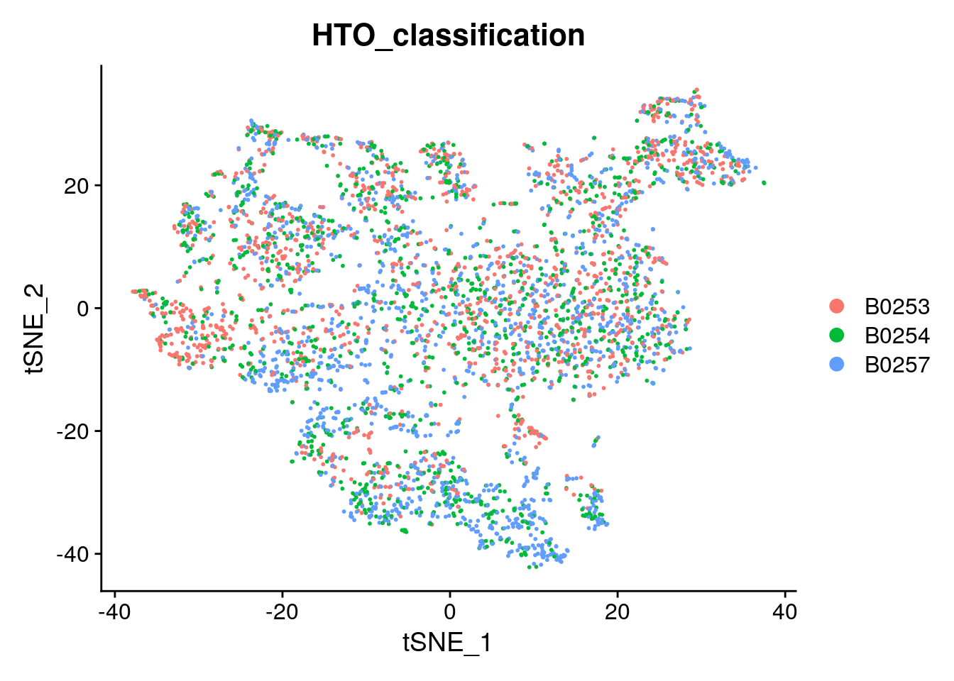
| Version | Author | Date |
|---|---|---|
| 4f37f3d | khembach | 2021-05-14 |
DimPlot(singlets, group.by = "HTO_classification", reduction = "umap")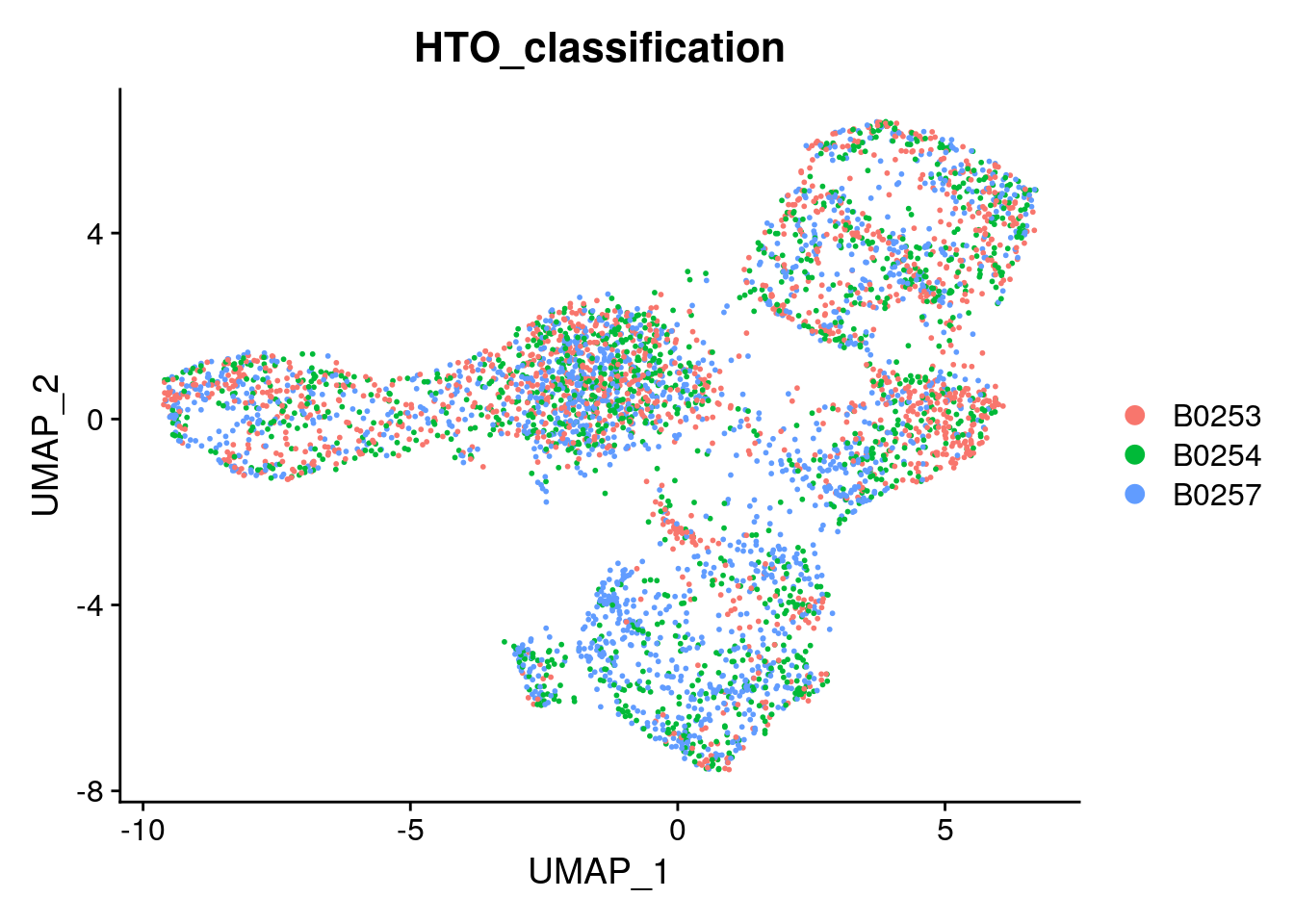
| Version | Author | Date |
|---|---|---|
| 4f37f3d | khembach | 2021-05-14 |
Identification of low quality cells
Based on the QC metrics, we identify cells with lower quality:
cols <- c("sum", "detected", "subsets_Mt_percent")
log <- c(TRUE, TRUE, FALSE)
type <- c("lower", "lower", "higher")

drop_cols <- paste0(cols, "_drop")
for (i in seq_along(cols))
    colData(sce)[[drop_cols[i]]] <- isOutlier(sce[[cols[i]]],
        nmads = 1, type = type[i], log = log[i], batch = sce$sample_id)

# Overlap of outlier cells from two metrics
sapply(drop_cols, function(i)
    sapply(drop_cols, function(j)
        sum(sce[[i]] & sce[[j]])))
sum_drop detected_drop subsets_Mt_percent_drop
sum_drop 0 0 0
detected_drop 0 53 49
subsets_Mt_percent_drop 0 49 3900colData(sce)$discard <- rowSums(data.frame(colData(sce)[,drop_cols])) > 0
table(colData(sce)$discard)
FALSE  TRUE
13727  3904
## Plot the metrics and highlight the discarded cells
plotColData(sce, x = "sample_id", y = "sum", colour_by = "discard") +
scale_y_log10()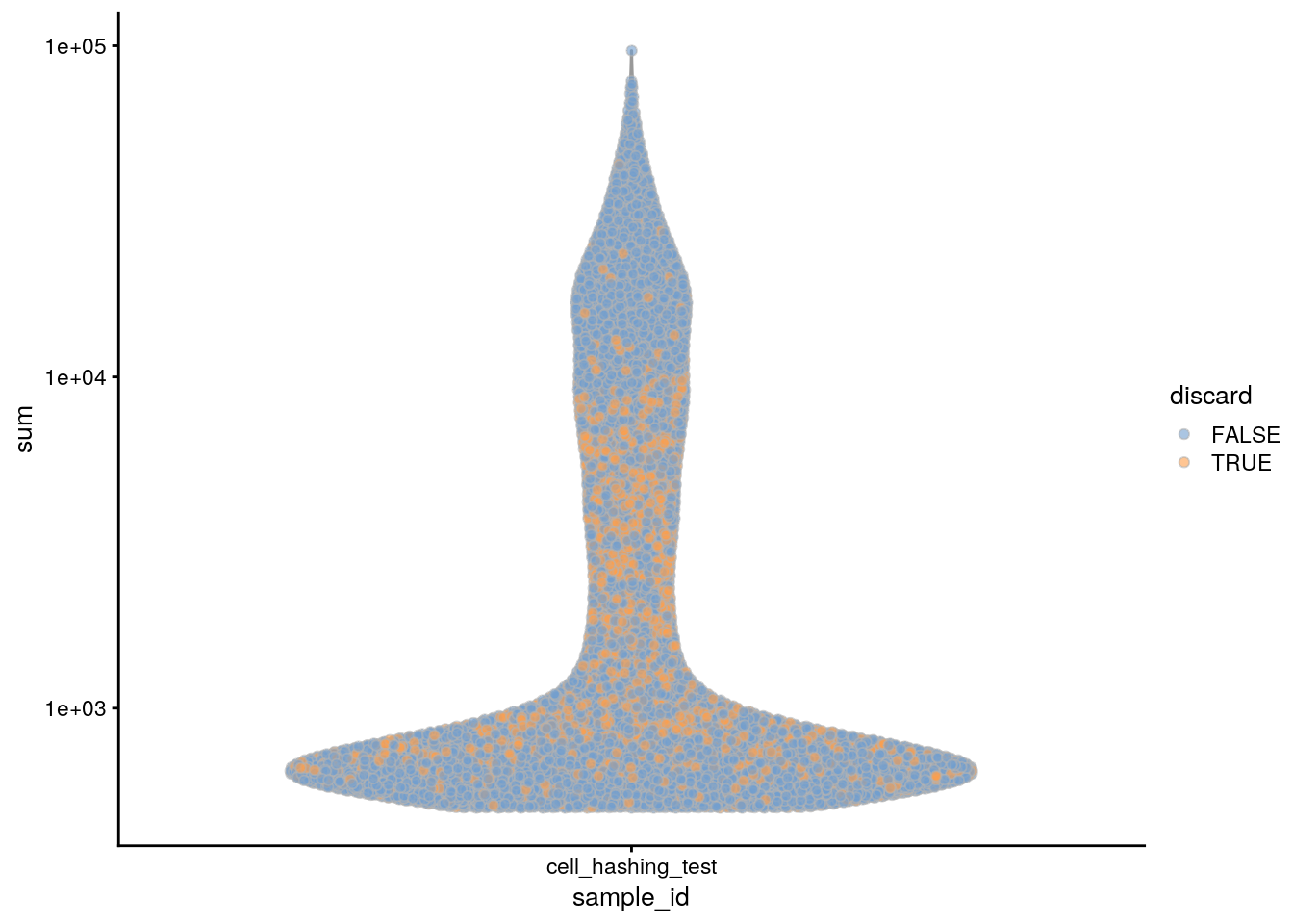
| Version | Author | Date |
|---|---|---|
| 4f37f3d | khembach | 2021-05-14 |
plotColData(sce, x = "sample_id", y = "detected", colour_by = "discard") +
  scale_y_log10()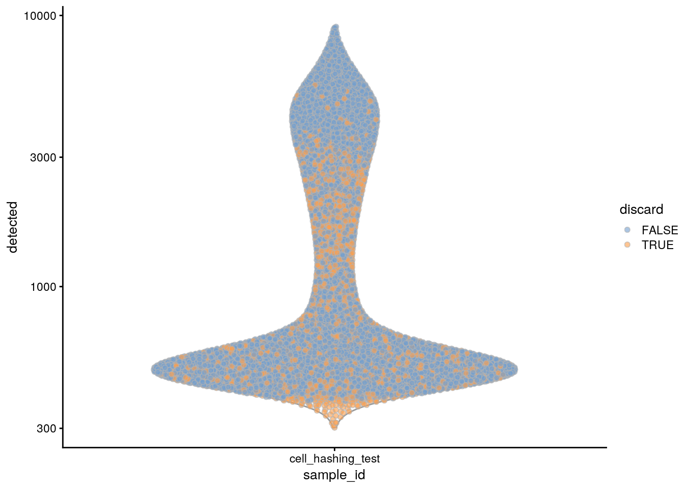
| Version | Author | Date |
|---|---|---|
| 4f37f3d | khembach | 2021-05-14 |
plotColData(sce, x = "sample_id", y = "subsets_Mt_percent",
            colour_by = "discard")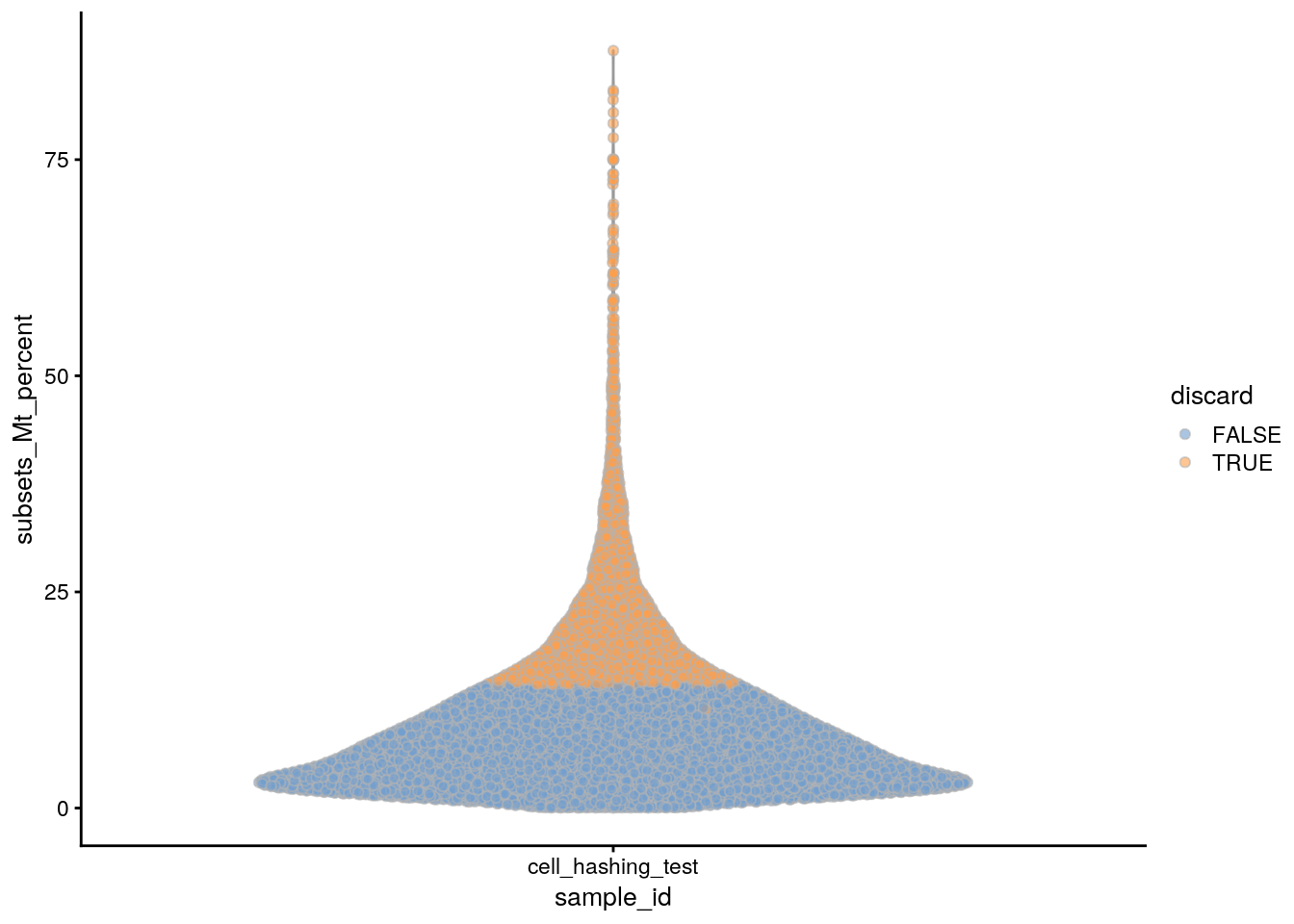
| Version | Author | Date |
|---|---|---|
| 4f37f3d | khembach | 2021-05-14 |
## we manually filter filter the cells with less than 2000 UMIs
colData(sce)$manual_discard_sum <- colData(sce)$sum < 1000
## filter the cells with less than 800 detected genes
colData(sce)$manual_discard_detected <- colData(sce)$detected < 800


## highlight all manually discarded cells
colData(sce)$manual_discard <- colData(sce)$manual_discard_sum |
                                   colData(sce)$manual_discard_detected
plotColData(sce, x = "sample_id", y = "sum", colour_by = "manual_discard") +
  scale_y_log10()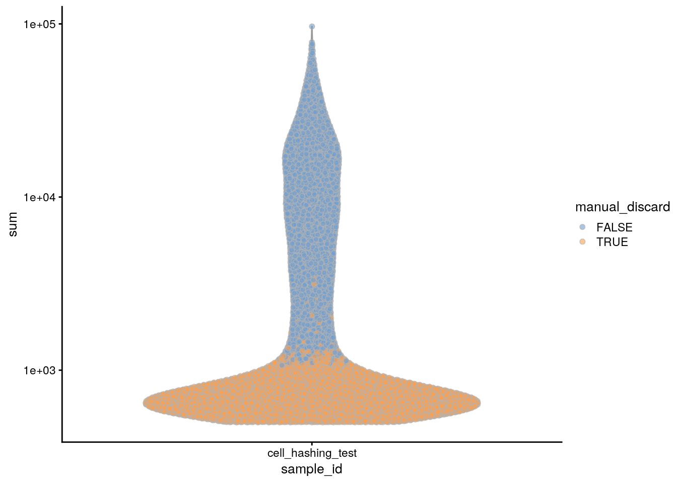
| Version | Author | Date |
|---|---|---|
| 4f37f3d | khembach | 2021-05-14 |
plotColData(sce, x = "sample_id", y = "detected", colour_by = "manual_discard") +
  scale_y_log10()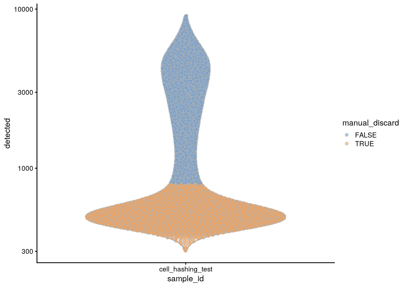
| Version | Author | Date |
|---|---|---|
| 4f37f3d | khembach | 2021-05-14 |
## highlight all discarded cells
colData(sce)$discard <- colData(sce)$manual_discard |
                                   colData(sce)$discard
plotColData(sce, x = "sample_id", y = "detected", colour_by = "discard") +
  scale_y_log10()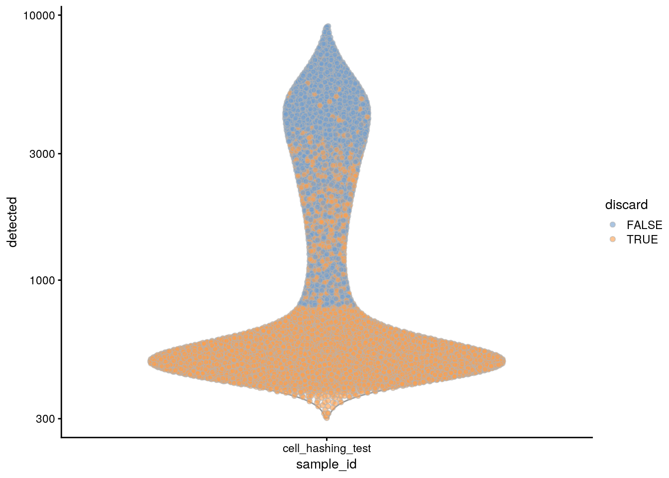
| Version | Author | Date |
|---|---|---|
| 4f37f3d | khembach | 2021-05-14 |
plotColData(sce, x = "sample_id", y = "sum", colour_by = "discard") +
  scale_y_log10()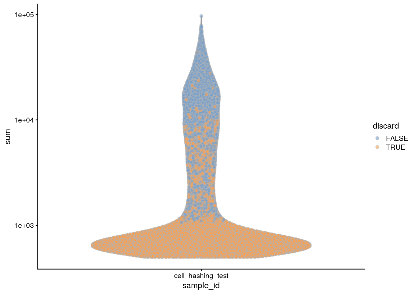
| Version | Author | Date |
|---|---|---|
| 4f37f3d | khembach | 2021-05-14 |
plotColData(sce, x = "sample_id", y = "subsets_Mt_percent",
            colour_by = "discard")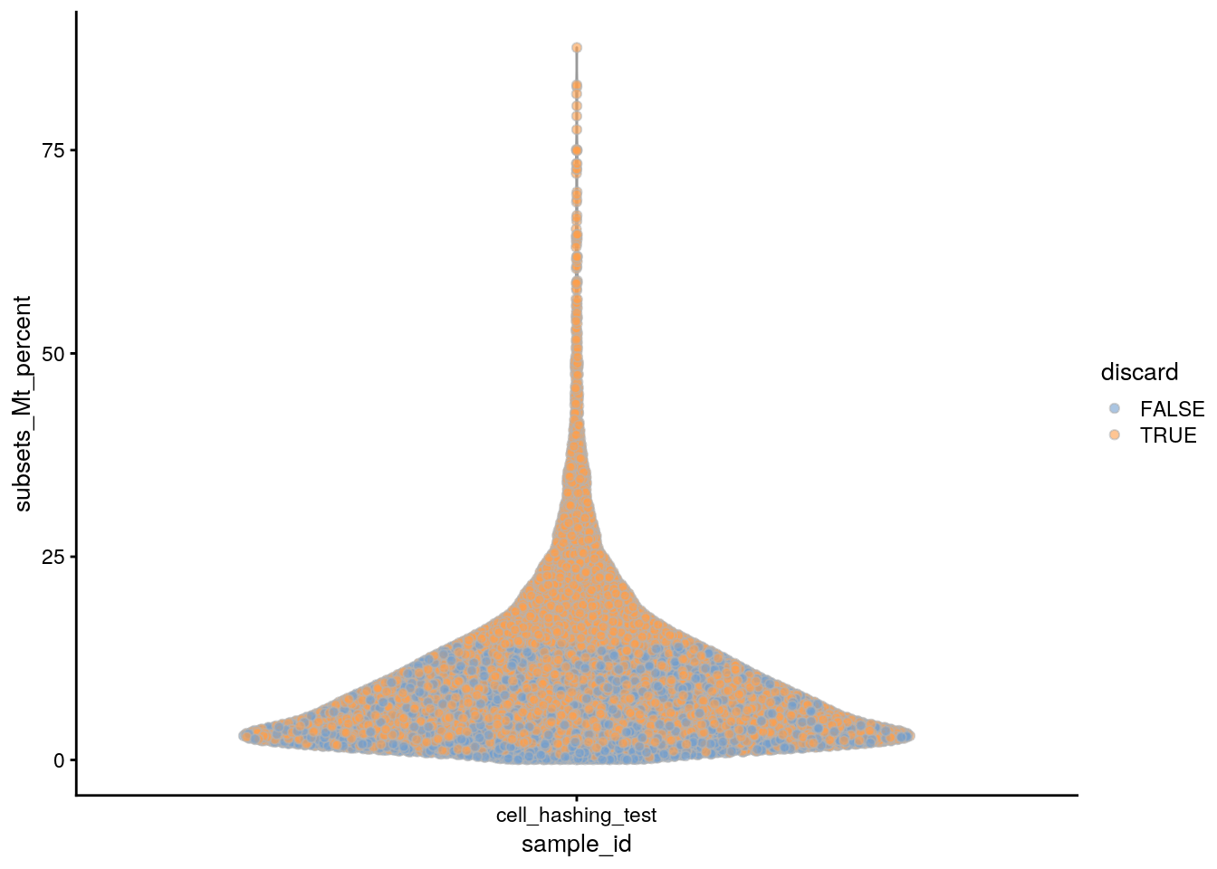
| Version | Author | Date |
|---|---|---|
| 4f37f3d | khembach | 2021-05-14 |
table(colData(sce)$discard)
FALSE  TRUE
 5542 12089
We discard the outlier cells
dim(sce)[1] 18824 17631sce_filtered <- sce[,!sce$discard]
dim(sce_filtered)[1] 18824 5542Create Seurat object and split gene and HTO counts
## convert DDelayedMatrix to dgCMatrix for import into Seurat object
counts <- as(counts(sce_filtered, withDimnames = FALSE), "dgCMatrix")
colnames(counts) <- colnames(counts(sce_filtered))
rownames(counts) <- rownames(counts(sce_filtered))

so_filtered <- CreateSeuratObject(
    counts = counts,
    meta.data = data.frame(colData(sce_filtered)),
    project = "cell_hashing_test")
Warning: Feature names cannot have underscores ('_'), replacing with dashes
('-')## add HTO data as independent assay
hto_counts <- as(counts(sce_raw, withDimnames = FALSE)[m,with(colData(sce),
paste(barcode, sample_id, sep = ".")) %in%
colnames(sce_filtered)], "dgCMatrix")
colnames(hto_counts) <- colnames(sce_filtered)
rownames(hto_counts) <- rownames(sce_raw)[m]
so_filtered[["HTO"]] <- CreateAssayObject(counts = hto_counts)Data normalization
DefaultAssay(so_filtered) <- "RNA"
# Normalize RNA data with log normalization
so_filtered <- NormalizeData(so_filtered)
# Find and scale variable features
so_filtered <- FindVariableFeatures(so_filtered, selection.method = "mean.var.plot")
so_filtered <- ScaleData(so_filtered, features = VariableFeatures(so_filtered))

# Normalize HTO data, here we use centered log-ratio (CLR) transformation
so_filtered <- NormalizeData(so_filtered, assay = "HTO", normalization.method = "CLR")
Demultiplex cells based on HTO enrichment
so_filtered <- HTODemux(so_filtered, assay = "HTO", positive.quantile = 0.99)Cutoff for B0253 : 801 readsCutoff for B0254 : 1097 readsCutoff for B0257 : 993 readsVisualize results
# Global classification results
table(so_filtered$HTO_classification.global)
 Doublet Negative  Singlet
     656     2119     2767
# Group cells based on the max HTO signal
Idents(so_filtered) <- "HTO_maxID"
# Group cells based on the max HTO signal
RidgePlot(so_filtered, assay = "HTO", features = rownames(so_filtered[["HTO"]]), ncol = 3)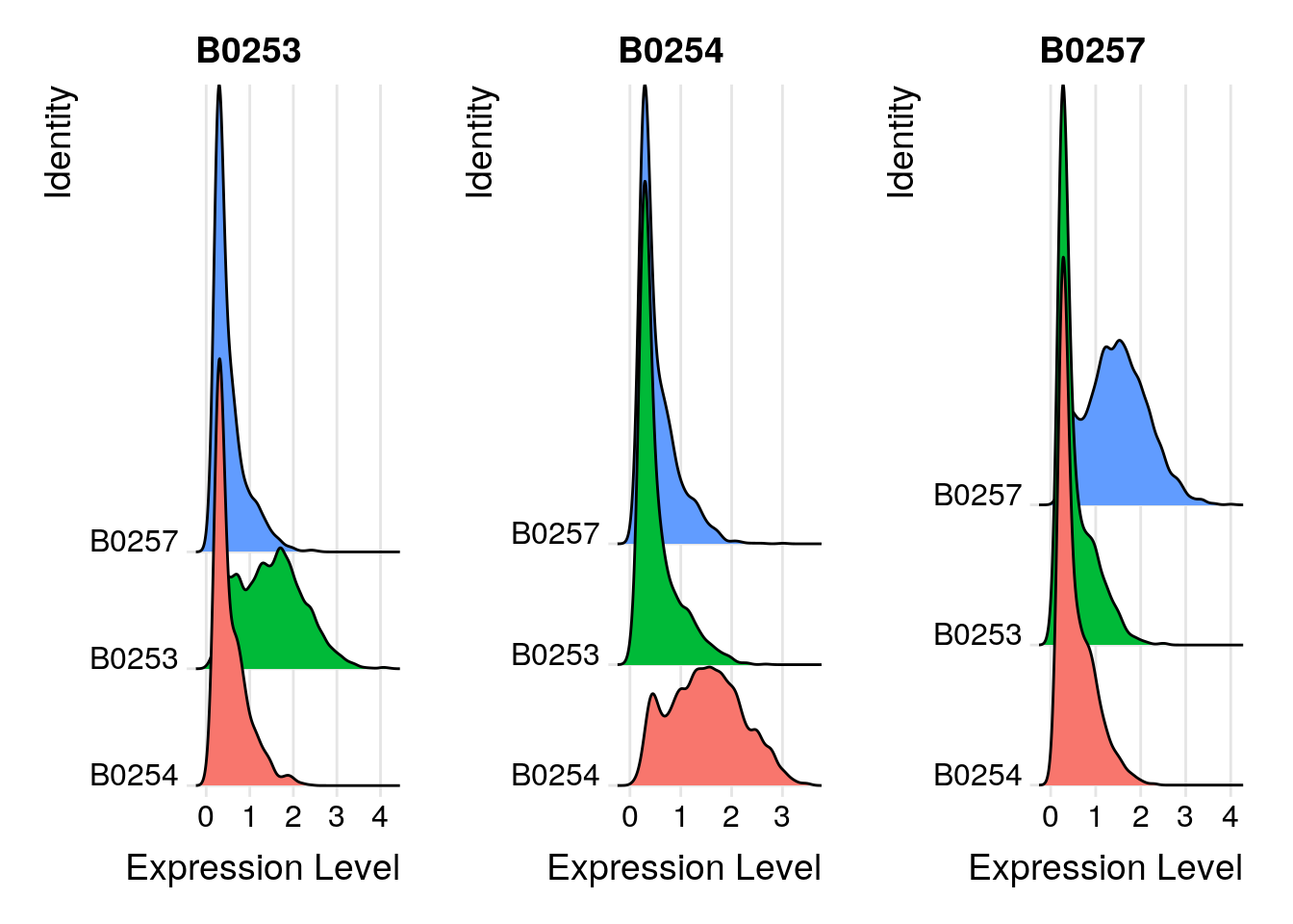
# Visualize pairs of HTO signals to check mutual exclusivity in singlets
DefaultAssay(object = so_filtered) <- "HTO"
FeatureScatter(so_filtered, feature1 = "B0253", feature2 = "B0254")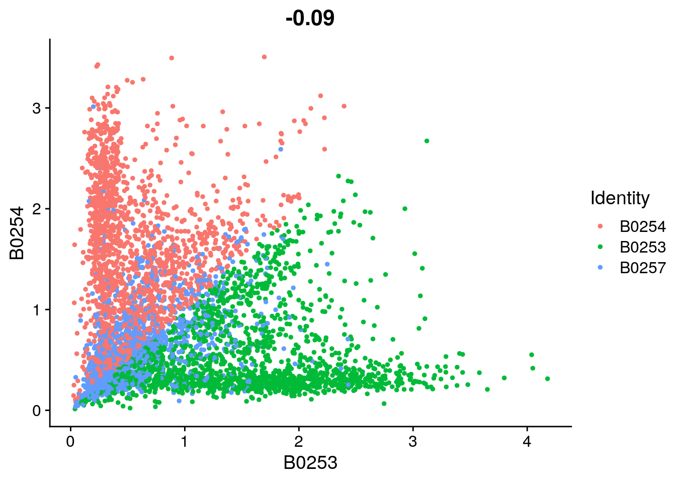
FeatureScatter(so_filtered, feature1 = "B0257", feature2 = "B0254")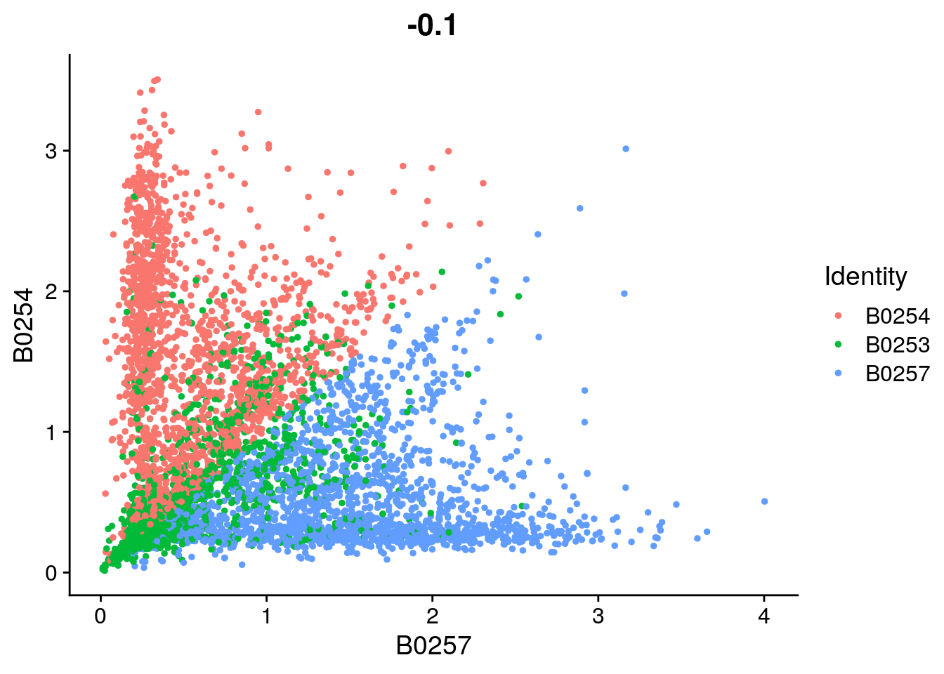
FeatureScatter(so_filtered, feature1 = "B0253", feature2 = "B0257")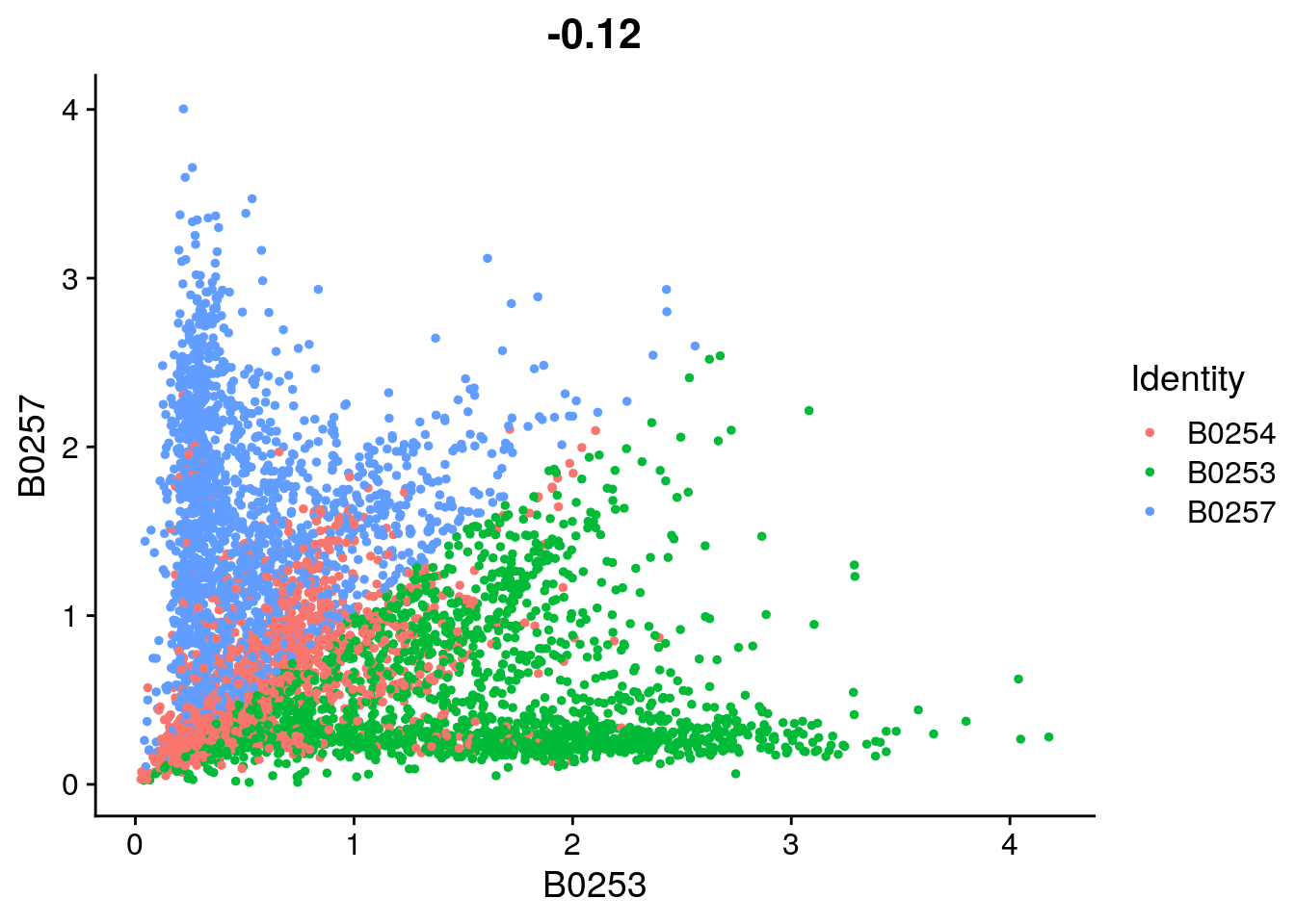
## compare number of UMIs for singlet's, doublets and negative cells
Idents(so_filtered) <- "HTO_classification.global"
VlnPlot(so_filtered, features = "nCount_HTO", pt.size = 0.1, log = TRUE)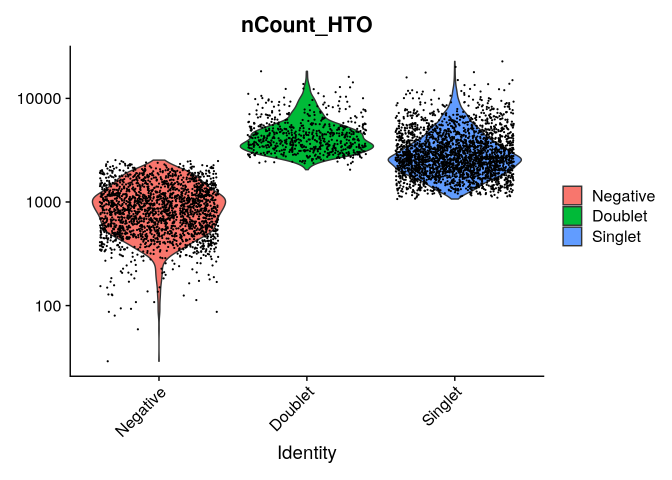
VlnPlot(so_filtered, features = "nCount_RNA", pt.size = 0.1, log = TRUE)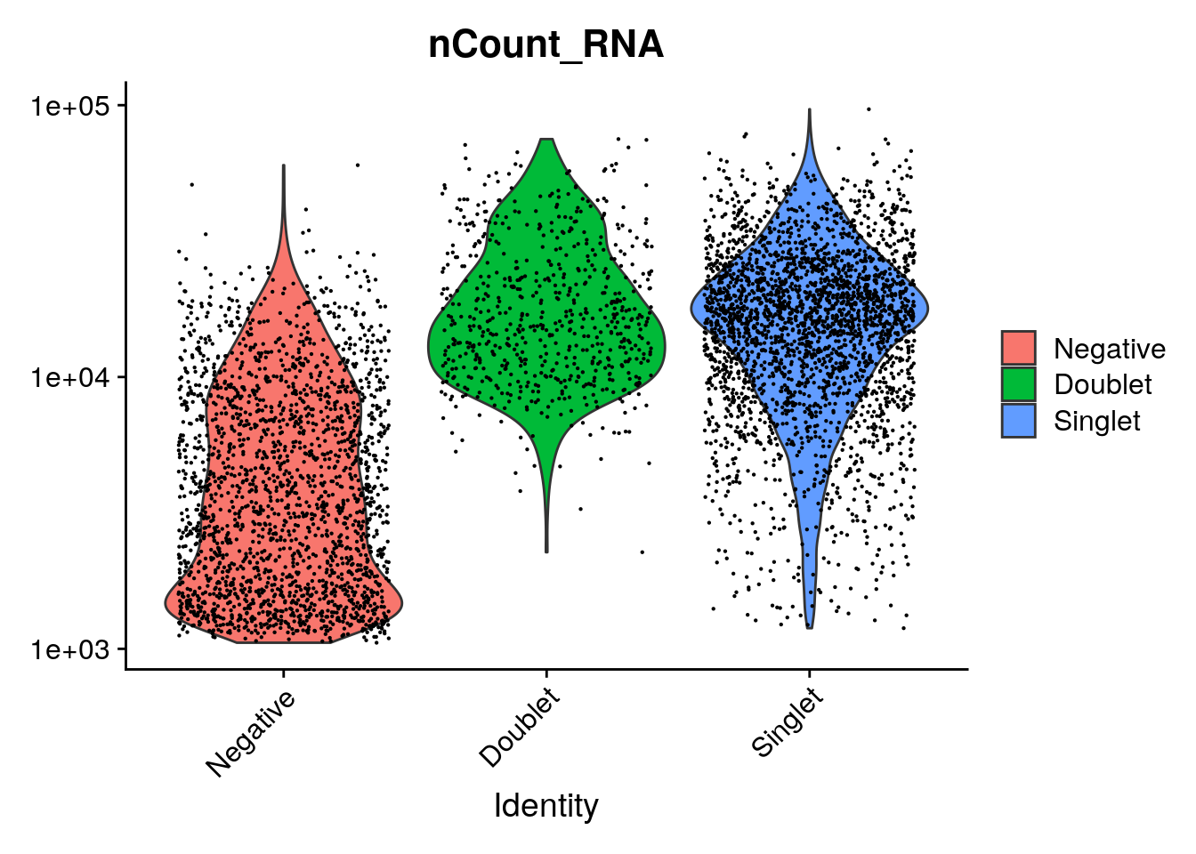
## tSNE for HTOs
# First, we will remove negative cells from the object
subs <- subset(so_filtered, idents = "Negative", invert = TRUE)
subs$HTO_classification %>% table
.
B0253 B0253_B0254 B0253_B0257 B0254 B0254_B0257 B0257
830 236 198 939 222 998 # Calculate a tSNE embedding of the HTO data
DefaultAssay(subs) <- "HTO"
subs <- ScaleData(subs, features = rownames(subs),
verbose = FALSE)
subs <- RunPCA(subs, features = rownames(subs), approx = FALSE, npcs = 3)Warning in print.DimReduc(x = reduction.data, dims = ndims.print, nfeatures =
nfeatures.print): Only 3 dimensions have been computed.Warning: Requested number is larger than the number of available items (3).
Setting to 3.
Warning: Requested number is larger than the number of available items (3).
Setting to 3.
Warning: Requested number is larger than the number of available items (3).
Setting to 3.subs <- RunTSNE(subs, dims = 1:3, perplexity = 100)
Idents(subs) <- "HTO_classification.global"
DimPlot(subs)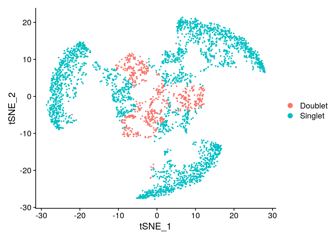
Idents(subs) <- 'HTO_classification'
DimPlot(subs)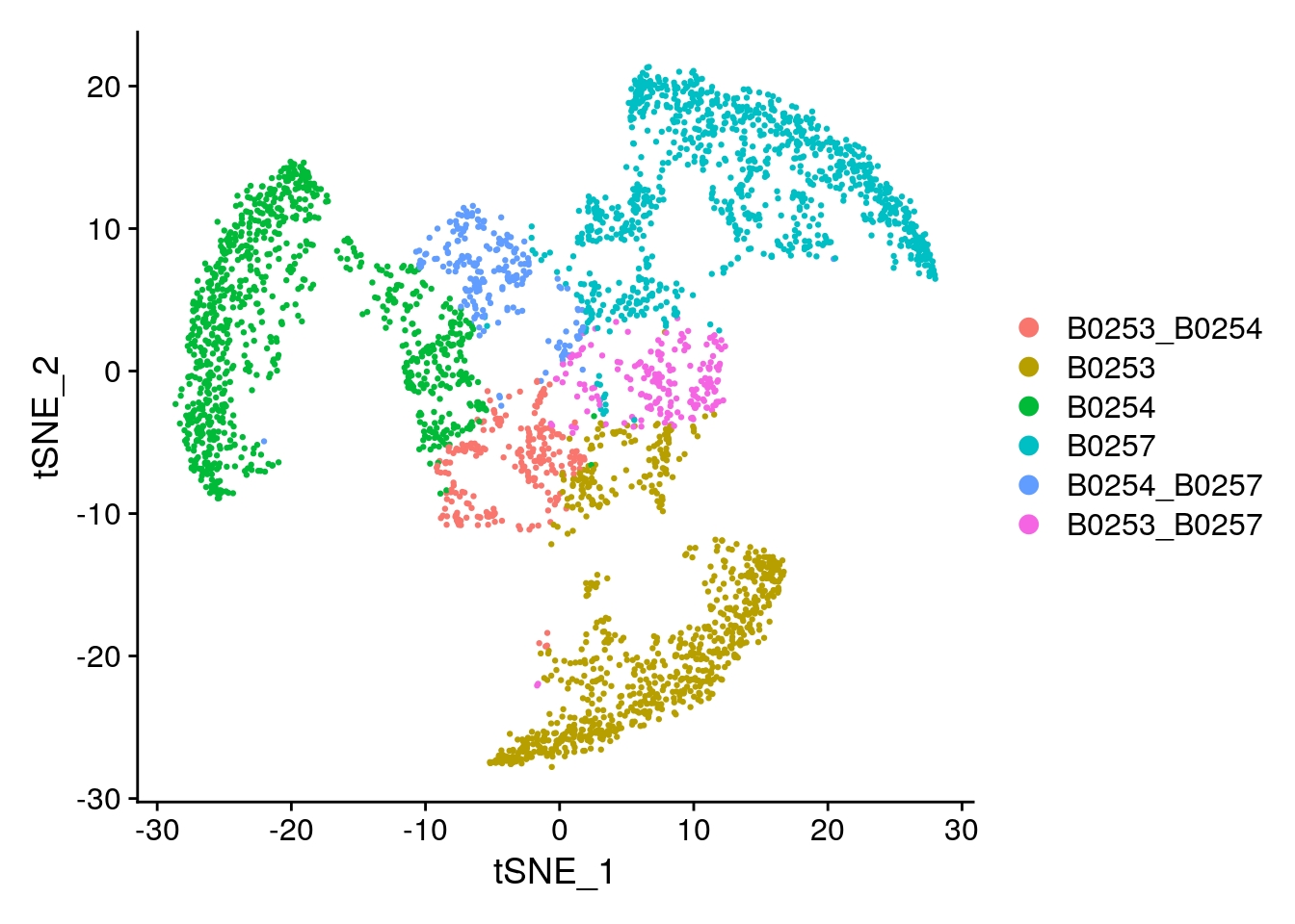
# HTO heatmap
HTOHeatmap(so_filtered, assay = "HTO", ncells = 5000)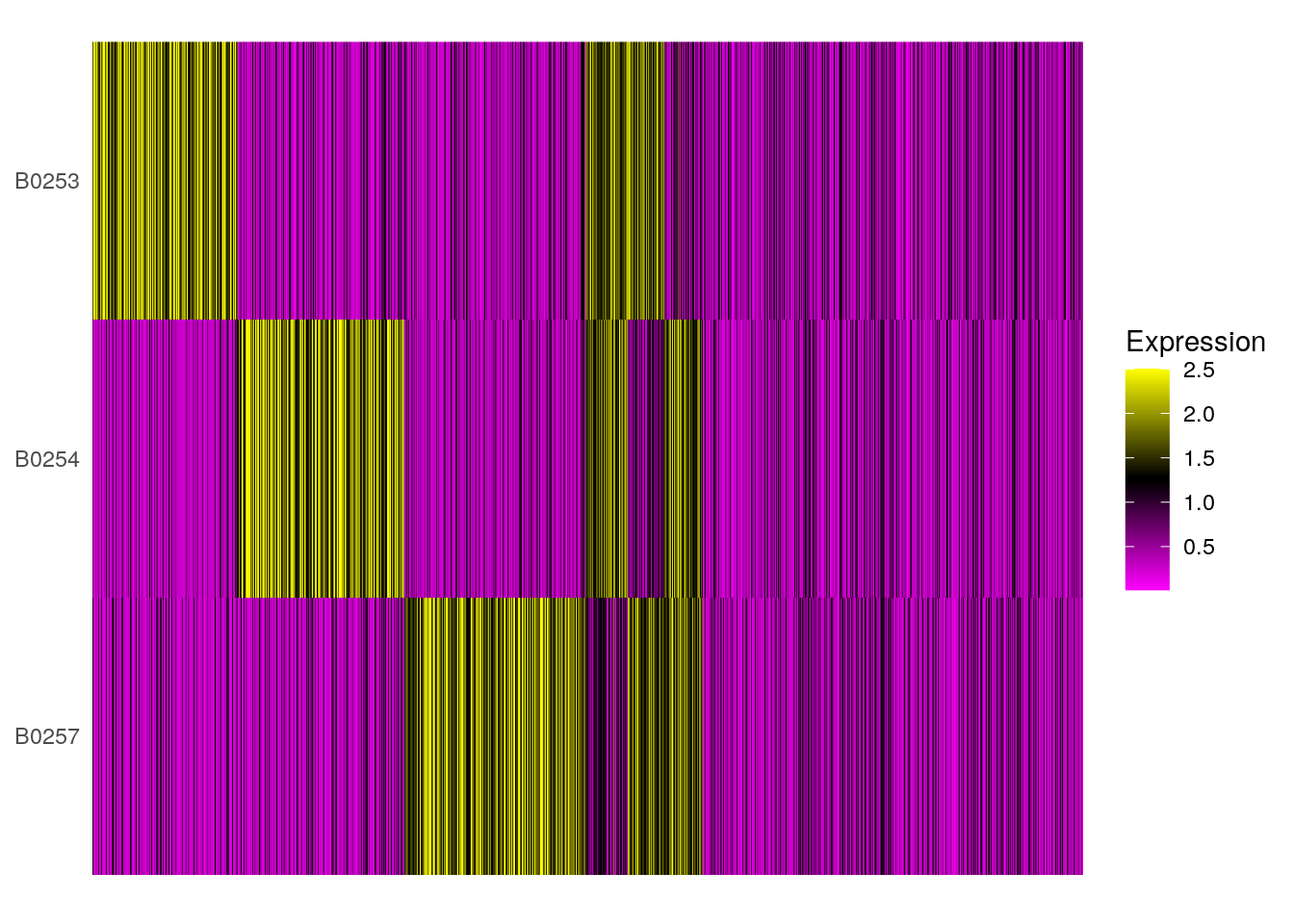
Cluster based on gene counts and visualize cells
DefaultAssay(so_filtered) <- "RNA"
# Extract the singlets
singlets_filtered <- subset(so_filtered, idents = "Singlet")
singlets_filtered$HTO_classification %>% table
.
B0253 B0254 B0257
830 939 998 # Select the top 1000 most variable features
singlets_filtered <- FindVariableFeatures(singlets_filtered, selection.method = "mean.var.plot")
# Scaling RNA data, we only scale the variable features here for efficiency
singlets_filtered <- ScaleData(singlets_filtered, features = VariableFeatures(singlets_filtered))
# Run PCA
singlets_filtered <- RunPCA(singlets_filtered, features = VariableFeatures(singlets_filtered))
# We select the top 10 PCs for clustering and tSNE based on PCElbowPlot
singlets_filtered <- FindNeighbors(singlets_filtered, reduction = "pca", dims = 1:10)
singlets_filtered <- FindClusters(singlets_filtered, resolution = 0.6, verbose = FALSE)
singlets_filtered <- RunTSNE(singlets_filtered, reduction = "pca", dims = 1:10)
singlets_filtered <- RunUMAP(singlets_filtered, reduction = "pca", dims = 1:10)
# Projecting singlet identities on TSNE visualization
DimPlot(singlets_filtered, group.by = "HTO_classification", reduction = "tsne")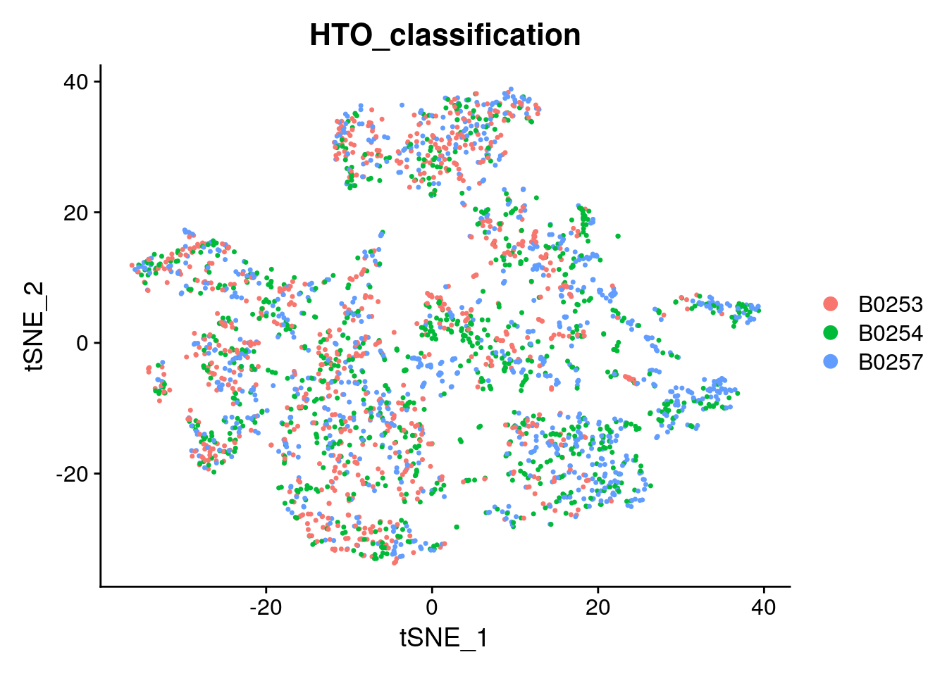
DimPlot(singlets_filtered, group.by = "HTO_classification", reduction = "umap")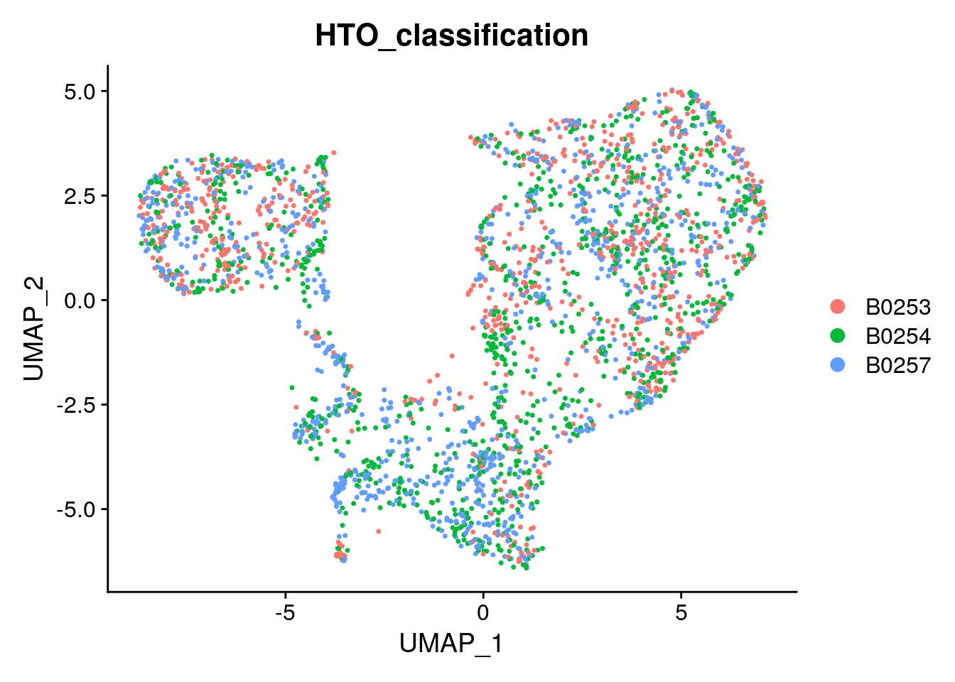
Save data to RDS
saveRDS(sce, file.path("output", "CH-test-01-preprocessing.rds"))
saveRDS(singlets, file.path("output", "CH-test-01-preprocessing_singlets.rds"))
saveRDS(so, file.path("output", "CH-test-01-preprocessing_so.rds"))
saveRDS(singlets_filtered, file.path("output", "CH-test-01-preprocessing_singlets_filtered.rds"))
saveRDS(so_filtered, file.path("output", "CH-test-01-preprocessing_so_filtered.rds"))
sessionInfo()R version 4.0.5 (2021-03-31)
Platform: x86_64-pc-linux-gnu (64-bit)
Running under: Ubuntu 18.04.5 LTS
Matrix products: default
BLAS: /usr/local/R/R-4.0.5/lib/libRblas.so
LAPACK: /usr/local/R/R-4.0.5/lib/libRlapack.so
locale:
[1] LC_CTYPE=en_US.UTF-8 LC_NUMERIC=C
[3] LC_TIME=en_US.UTF-8 LC_COLLATE=en_US.UTF-8
[5] LC_MONETARY=en_US.UTF-8 LC_MESSAGES=en_US.UTF-8
[7] LC_PAPER=en_US.UTF-8 LC_NAME=C
[9] LC_ADDRESS=C LC_TELEPHONE=C
[11] LC_MEASUREMENT=en_US.UTF-8 LC_IDENTIFICATION=C
attached base packages:
[1] parallel stats4 stats graphics grDevices utils datasets
[8] methods base
other attached packages:
[1] dplyr_1.0.2 viridis_0.5.1
[3] viridisLite_0.3.0 scales_1.1.1
[5] SeuratObject_4.0.1 Seurat_4.0.1
[7] readxl_1.3.1 scater_1.16.2
[9] ggplot2_3.3.2 BiocParallel_1.22.0
[11] DropletUtils_1.8.0 SingleCellExperiment_1.10.1
[13] SummarizedExperiment_1.18.1 DelayedArray_0.14.0
[15] matrixStats_0.56.0 Biobase_2.48.0
[17] GenomicRanges_1.40.0 GenomeInfoDb_1.24.2
[19] IRanges_2.22.2 S4Vectors_0.26.1
[21] BiocGenerics_0.34.0 workflowr_1.6.2
loaded via a namespace (and not attached):
[1] backports_1.1.9 plyr_1.8.6
[3] igraph_1.2.5 lazyeval_0.2.2
[5] splines_4.0.5 listenv_0.8.0
[7] scattermore_0.7 digest_0.6.25
[9] htmltools_0.5.0 magrittr_1.5
[11] tensor_1.5 cluster_2.1.0
[13] ROCR_1.0-11 limma_3.44.3
[15] globals_0.12.5 R.utils_2.9.2
[17] spatstat.sparse_2.0-0 colorspace_1.4-1
[19] rappdirs_0.3.1 ggrepel_0.8.2
[21] xfun_0.15 crayon_1.3.4
[23] RCurl_1.98-1.3 jsonlite_1.7.2
[25] spatstat.data_2.1-0 survival_3.2-3
[27] zoo_1.8-8 glue_1.4.2
[29] polyclip_1.10-0 gtable_0.3.0
[31] zlibbioc_1.34.0 XVector_0.28.0
[33] leiden_0.3.3 BiocSingular_1.4.0
[35] Rhdf5lib_1.10.0 future.apply_1.6.0
[37] HDF5Array_1.16.1 abind_1.4-5
[39] edgeR_3.30.3 miniUI_0.1.1.1
[41] Rcpp_1.0.5 isoband_0.2.2
[43] xtable_1.8-4 reticulate_1.16
[45] spatstat.core_2.1-2 dqrng_0.2.1
[47] rsvd_1.0.3 htmlwidgets_1.5.1
[49] httr_1.4.2 RColorBrewer_1.1-2
[51] ellipsis_0.3.1 ica_1.0-2
[53] farver_2.0.3 pkgconfig_2.0.3
[55] R.methodsS3_1.8.0 uwot_0.1.10
[57] deldir_0.2-10 locfit_1.5-9.4
[59] labeling_0.3 tidyselect_1.1.0
[61] rlang_0.4.10 reshape2_1.4.4
[63] later_1.1.0.1 munsell_0.5.0
[65] cellranger_1.1.0 tools_4.0.5
[67] generics_0.0.2 ggridges_0.5.2
[69] evaluate_0.14 stringr_1.4.0
[71] fastmap_1.0.1 goftest_1.2-2
[73] yaml_2.2.1 knitr_1.29
[75] fs_1.5.0 fitdistrplus_1.1-1
[77] purrr_0.3.4 RANN_2.6.1
[79] nlme_3.1-148 pbapply_1.4-2
[81] future_1.17.0 whisker_0.4
[83] mime_0.9 R.oo_1.23.0
[85] compiler_4.0.5 beeswarm_0.2.3
[87] plotly_4.9.2.1 png_0.1-7
[89] spatstat.utils_2.1-0 tibble_3.0.3
[91] stringi_1.4.6 RSpectra_0.16-0
[93] lattice_0.20-41 Matrix_1.3-3
[95] vctrs_0.3.4 pillar_1.4.6
[97] lifecycle_1.0.0 spatstat.geom_2.1-0
[99] lmtest_0.9-37 RcppAnnoy_0.0.18
[101] BiocNeighbors_1.6.0 data.table_1.12.8
[103] cowplot_1.0.0 bitops_1.0-6
[105] irlba_2.3.3 httpuv_1.5.4
[107] patchwork_1.0.1 R6_2.4.1
[109] promises_1.1.1 KernSmooth_2.23-17
[111] gridExtra_2.3 vipor_0.4.5
[113] codetools_0.2-16 MASS_7.3-51.6
[115] rhdf5_2.32.2 rprojroot_1.3-2
[117] withr_2.4.1 sctransform_0.3.2
[119] GenomeInfoDbData_1.2.3 mgcv_1.8-31
[121] beachmat_2.4.0 rpart_4.1-15
[123] grid_4.0.5 tidyr_1.1.0
[125] rmarkdown_2.3 DelayedMatrixStats_1.10.1
[127] Rtsne_0.15 git2r_0.27.1
[129] shiny_1.5.0 ggbeeswarm_0.6.0