Cluster annotation
Katharina Hembach
5/29/2020
Last updated: 2020-06-26
Checks: 7 0
Knit directory: neural_scRNAseq/
This reproducible R Markdown analysis was created with workflowr (version 1.6.2). The Checks tab describes the reproducibility checks that were applied when the results were created. The Past versions tab lists the development history.
Great! Since the R Markdown file has been committed to the Git repository, you know the exact version of the code that produced these results.
Great job! The global environment was empty. Objects defined in the global environment can affect the analysis in your R Markdown file in unknown ways. For reproduciblity it’s best to always run the code in an empty environment.
The command set.seed(20200522) was run prior to running the code in the R Markdown file. Setting a seed ensures that any results that rely on randomness, e.g. subsampling or permutations, are reproducible.
Great job! Recording the operating system, R version, and package versions is critical for reproducibility.
Nice! There were no cached chunks for this analysis, so you can be confident that you successfully produced the results during this run.
Great job! Using relative paths to the files within your workflowr project makes it easier to run your code on other machines.
Great! You are using Git for version control. Tracking code development and connecting the code version to the results is critical for reproducibility.
The results in this page were generated with repository version afe57cc. See the Past versions tab to see a history of the changes made to the R Markdown and HTML files.
Note that you need to be careful to ensure that all relevant files for the analysis have been committed to Git prior to generating the results (you can use wflow_publish or wflow_git_commit). workflowr only checks the R Markdown file, but you know if there are other scripts or data files that it depends on. Below is the status of the Git repository when the results were generated:
Ignored files:
    Ignored:    .DS_Store
    Ignored:    .Rhistory
    Ignored:    .Rproj.user/
    Ignored:    ._.DS_Store
    Ignored:    ._MA.pdf
    Ignored:    ._MA2.pdf
    Ignored:    ._MA_plots.pdf
    Ignored:    ._Rplots.pdf
    Ignored:    .__workflowr.yml
    Ignored:    ._hm.pdf
    Ignored:    ._neural_scRNAseq.Rproj
    Ignored:    ._sample5_MA_2nd_pop.pdf
    Ignored:    ._sample5_QC_2nd_pop.pdf
    Ignored:    ._tmp.pdf
    Ignored:    ._tmp_detected.pdf
    Ignored:    ._tmp_manual_discard.pdf
    Ignored:    ._tmp_manual_discard1.pdf
    Ignored:    ._tmp_manual_discard_all.pdf
    Ignored:    ._tmp_manual_discard_all1.pdf
    Ignored:    analysis/.DS_Store
    Ignored:    analysis/.Rhistory
    Ignored:    analysis/._.DS_Store
    Ignored:    analysis/._01-preprocessing.Rmd
    Ignored:    analysis/._01-preprocessing.html
    Ignored:    analysis/._02.1-SampleQC.Rmd
    Ignored:    analysis/._03-filtering.Rmd
    Ignored:    analysis/._04-clustering.Rmd
    Ignored:    analysis/._04-clustering.knit.md
    Ignored:    analysis/._04.1-cell_cycle.Rmd
    Ignored:    analysis/._05-annotation.Rmd
    Ignored:    analysis/.__site.yml
    Ignored:    analysis/._additional_filtering.Rmd
    Ignored:    analysis/._additional_filtering_clustering.Rmd
    Ignored:    analysis/._index.Rmd
    Ignored:    analysis/01-preprocessing_cache/
    Ignored:    analysis/02-1-SampleQC_cache/
    Ignored:    analysis/02-quality_control_cache/
    Ignored:    analysis/02.1-SampleQC_cache/
    Ignored:    analysis/03-filtering_cache/
    Ignored:    analysis/04-clustering_cache/
    Ignored:    analysis/04.1-cell_cycle_cache/
    Ignored:    analysis/additional_filtering_cache/
    Ignored:    analysis/additional_filtering_clustering_cache/
    Ignored:    analysis/sample5_QC_cache/
    Ignored:    data/.DS_Store
    Ignored:    data/._.DS_Store
    Ignored:    data/._.smbdeleteAAA17ed8b4b
    Ignored:    data/._metadata.csv
    Ignored:    data/data_sushi/
    Ignored:    data/filtered_feature_matrices/
    Ignored:    output/.DS_Store
    Ignored:    output/._.DS_Store
    Ignored:    output/additional_filtering.rds
    Ignored:    output/figures/
    Ignored:    output/sce_01_preprocessing.rds
    Ignored:    output/sce_02_quality_control.rds
    Ignored:    output/sce_03_filtering.rds
    Ignored:    output/sce_preprocessing.rds
    Ignored:    output/so_04_1_cell_cycle.rds
    Ignored:    output/so_04_clustering.rds
    Ignored:    output/so_additional_filtering_clustering.rds

Untracked files:
    Untracked:  MA.pdf
    Untracked:  MA2.pdf
    Untracked:  MA_plots.pdf
    Untracked:  Rplots.pdf
    Untracked:  analysis/additional_filtering.Rmd
    Untracked:  analysis/additional_filtering_clustering.Rmd
    Untracked:  analysis/sample5_QC.Rmd
    Untracked:  analysis/tabsets.Rmd
    Untracked:  hm.pdf
    Untracked:  sample5_MA_2nd_pop.pdf
    Untracked:  sample5_QC_2nd_pop.pdf
    Untracked:  scripts/
    Untracked:  tmp.pdf
    Untracked:  tmp_detected.pdf
    Untracked:  tmp_manual_discard.pdf
    Untracked:  tmp_manual_discard1.pdf
    Untracked:  tmp_manual_discard_all.pdf
    Untracked:  tmp_manual_discard_all1.pdf

Unstaged changes:
    Modified:   analysis/_site.yml
Note that any generated files, e.g. HTML, png, CSS, etc., are not included in this status report because it is ok for generated content to have uncommitted changes.
These are the previous versions of the repository in which changes were made to the R Markdown (analysis/05-annotation.Rmd) and HTML (docs/05-annotation.html) files. If you’ve configured a remote Git repository (see ?wflow_git_remote), click on the hyperlinks in the table below to view the files as they were in that past version.
| File | Version | Author | Date | Message |
|---|---|---|---|---|
| html | 06330b1 | khembach | 2020-06-22 | Build site. |
| Rmd | f349423 | khembach | 2020-06-21 | regress out number of UMIs and perc mitochondrial features; cyclone |
| html | 4e52d16 | khembach | 2020-06-15 | Build site. |
| Rmd | 47f9578 | khembach | 2020-06-15 | fix tabset |
| html | d04635a | khembach | 2020-06-12 | Build site. |
| Rmd | f376d76 | khembach | 2020-06-12 | add barplot with sample fraction to heatmap |
| html | 34b86b8 | khembach | 2020-06-12 | Build site. |
| Rmd | 38c33d8 | khembach | 2020-06-12 | do not print marker ids |
| html | 98d3f0d | khembach | 2020-06-12 | Build site. |
| Rmd | a8f31cd | khembach | 2020-06-12 | analyze known marker genes |
| html | f116d0f | khembach | 2020-06-10 | Build site. |
| Rmd | b6767a6 | khembach | 2020-06-10 | wflow_publish(“analysis/05-annotation.Rmd”, verbose = TRUE) |
| html | 419ac73 | khembach | 2020-06-09 | Build site. |
| html | a4d0e04 | khembach | 2020-05-29 | Build site. |
| Rmd | 97d5a52 | khembach | 2020-05-29 | cluster analysis |
Load packages
library(ComplexHeatmap)
library(cowplot)
library(ggplot2)
library(dplyr)
library(muscat)
library(purrr)
library(RColorBrewer)
library(viridis)
library(scran)
library(Seurat)
library(SingleCellExperiment)
library(stringr)
library(RCurl)
library(BiocParallel)
Load data & convert to SCE
so <- readRDS(file.path("output", "so_04_clustering.rds"))
sce <- as.SingleCellExperiment(so, assay = "RNA")
colData(sce) <- as.data.frame(colData(sce)) %>%
    mutate_if(is.character, as.factor) %>%
    DataFrame(row.names = colnames(sce))
Number of clusters by resolution
cluster_cols <- grep("res.[0-9]", colnames(colData(sce)), value = TRUE)
sapply(colData(sce)[cluster_cols], nlevels)
integrated_snn_res.0.1 integrated_snn_res.0.2 integrated_snn_res.0.4
9 10 17
integrated_snn_res.0.8 integrated_snn_res.1 integrated_snn_res.1.2
23 28 30
integrated_snn_res.2
35 Cluster-sample counts
# set cluster IDs to resolution 0.4 clustering
so <- SetIdent(so, value = "integrated_snn_res.0.4")
so@meta.data$cluster_id <- Idents(so)
sce$cluster_id <- Idents(so)
(n_cells <- table(sce$cluster_id, sce$sample_id))
     1NSC 2NSC 3NC52 4NC52 5NC96 6NC96
  0  5184 5397   238   107   152   116
  1     0    1  1602  1312   447   576
  2  1430 1273    69    55    18    11
  3   753  727   301   279   340   363
  4     4    5   653   676   500   770
  5     1    1   970   870   265   374
  6     0    0   979   818   256   414
  7     0    0   912   781   270   369
  8   159  149   541   578   235   286
  9     0    0   793   613   209   255
  10  426  474   117   108    94   121
  11  243  237   203   261   178   206
  12    3    2   400   270   236   265
  13    0    1   395   277   127   176
  14   12    9   315   251   137   191
  15   32   45   150   138    40    83
  16   84   87    49    44    34    19
Relative cluster-abundances
fqs <- prop.table(n_cells, margin = 2)
mat <- as.matrix(unclass(fqs))
Heatmap(mat,
    col = rev(brewer.pal(11, "RdGy")[-6]),
    name = "Frequency",
    cluster_rows = FALSE,
    cluster_columns = FALSE,
    row_names_side = "left",
    row_title = "cluster_id",
    column_title = "sample_id",
    column_title_side = "bottom",
    rect_gp = gpar(col = "white"),
    cell_fun = function(i, j, x, y, width, height, fill)
        grid.text(round(mat[j, i] * 100, 2), x = x, y = y,
            gp = gpar(col = "white", fontsize = 8)))
Cell cycle scoring with Seurat
We assign each cell a cell cycle scores and visualize them in the DR plots. We use known G2/M and S phase markers that come with the Seurat package. The markers are anticorrelated and cells that to not express the markers should be in G1 phase.
We compute cell cycle phase:
DefaultAssay(so) <- "RNA"
# A list of cell cycle markers, from Tirosh et al, 2015
cc_file <- getURL("https://raw.githubusercontent.com/hbc/tinyatlas/master/cell_cycle/Homo_sapiens.csv")
cc_genes <- read.csv(text = cc_file)
# match the marker genes to the features
m <- match(cc_genes$geneID[cc_genes$phase == "S"],
           str_split(rownames(GetAssayData(so)),
                     pattern = "\\.", simplify = TRUE)[,1])
s_genes <- rownames(GetAssayData(so))[m]
(s_genes <- s_genes[!is.na(s_genes)])
[1] "ENSG00000012963.UBR7" "ENSG00000049541.RFC2"
[3] "ENSG00000051180.RAD51" "ENSG00000073111.MCM2"
[5] "ENSG00000075131.TIPIN" "ENSG00000076003.MCM6"
[7] "ENSG00000076248.UNG" "ENSG00000077514.POLD3"
[9] "ENSG00000092470.WDR76" "ENSG00000092853.CLSPN"
[11] "ENSG00000093009.CDC45" "ENSG00000094804.CDC6"
[13] "ENSG00000095002.MSH2" "ENSG00000100297.MCM5"
[15] "ENSG00000101868.POLA1" "ENSG00000104738.MCM4"
[17] "ENSG00000111247.RAD51AP1" "ENSG00000112312.GMNN"
[19] "ENSG00000117748.RPA2" "ENSG00000118412.CASP8AP2"
[21] "ENSG00000119969.HELLS" "ENSG00000129173.E2F8"
[23] "ENSG00000131153.GINS2" "ENSG00000132646.PCNA"
[25] "ENSG00000132780.NASP" "ENSG00000136492.BRIP1"
[27] "ENSG00000136982.DSCC1" "ENSG00000143476.DTL"
[29] "ENSG00000144354.CDCA7" "ENSG00000151725.CENPU"
[31] "ENSG00000156802.ATAD2" "ENSG00000159259.CHAF1B"
[33] "ENSG00000162607.USP1" "ENSG00000163950.SLBP"
[35] "ENSG00000167325.RRM1" "ENSG00000168496.FEN1"
[37] "ENSG00000171848.RRM2" "ENSG00000174371.EXO1"
[39] "ENSG00000175305.CCNE2" "ENSG00000176890.TYMS"
[41] "ENSG00000197299.BLM" "ENSG00000198056.PRIM1"
[43] "ENSG00000276043.UHRF1" m <- match(cc_genes$geneID[cc_genes$phase == "G2/M"],
str_split(rownames(GetAssayData(so)),
pattern = "\\.", simplify = TRUE)[,1])
g2m_genes <- rownames(GetAssayData(so))[m]
(g2m_genes <- g2m_genes[!is.na(g2m_genes)]) [1] "ENSG00000010292.NCAPD2" "ENSG00000011426.ANLN"
[3] "ENSG00000013810.TACC3" "ENSG00000072571.HMMR"
[5] "ENSG00000075218.GTSE1" "ENSG00000080986.NDC80"
[7] "ENSG00000087586.AURKA" "ENSG00000088325.TPX2"
[9] "ENSG00000089685.BIRC5" "ENSG00000092140.G2E3"
[11] "ENSG00000094916.CBX5" "ENSG00000100401.RANGAP1"
[13] "ENSG00000102974.CTCF" "ENSG00000111665.CDCA3"
[15] "ENSG00000112742.TTK" "ENSG00000113810.SMC4"
[17] "ENSG00000114346.ECT2" "ENSG00000115163.CENPA"
[19] "ENSG00000117399.CDC20" "ENSG00000117650.NEK2"
[21] "ENSG00000117724.CENPF" "ENSG00000120802.TMPO"
[23] "ENSG00000123485.HJURP" "ENSG00000123975.CKS2"
[25] "ENSG00000126787.DLGAP5" "ENSG00000129195.PIMREG"
[27] "ENSG00000131747.TOP2A" "ENSG00000134222.PSRC1"
[29] "ENSG00000134690.CDCA8" "ENSG00000136108.CKAP2"
[31] "ENSG00000137804.NUSAP1" "ENSG00000137807.KIF23"
[33] "ENSG00000138160.KIF11" "ENSG00000138182.KIF20B"
[35] "ENSG00000138778.CENPE" "ENSG00000139354.GAS2L3"
[37] "ENSG00000142945.KIF2C" "ENSG00000143228.NUF2"
[39] "ENSG00000143401.ANP32E" "ENSG00000143815.LBR"
[41] "ENSG00000148773.MKI67" "ENSG00000157456.CCNB2"
[43] "ENSG00000158402.CDC25C" "ENSG00000164104.HMGB2"
[45] "ENSG00000169607.CKAP2L" "ENSG00000169679.BUB1"
[47] "ENSG00000170312.CDK1" "ENSG00000173207.CKS1B"
[49] "ENSG00000175063.UBE2C" "ENSG00000175216.CKAP5"
[51] "ENSG00000178999.AURKB" "ENSG00000184661.CDCA2"
[53] "ENSG00000188229.TUBB4B" "ENSG00000189159.JPT1" so <- CellCycleScoring(so, s.features = s_genes, g2m.features = g2m_genes,
set.ident = TRUE)
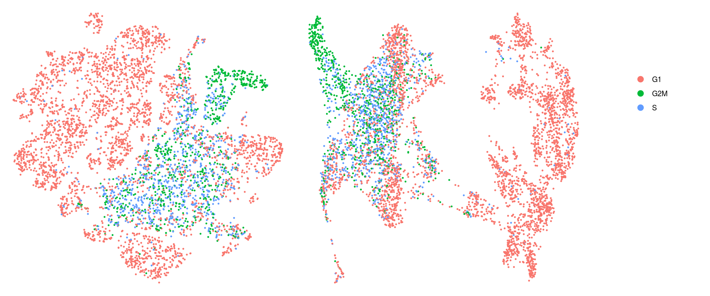
DefaultAssay(so) <- "integrated"DR colored by cluster ID
cs <- sample(colnames(so), 5e3)
.plot_dr <- function(so, dr, id)
    DimPlot(so, cells = cs, group.by = id, reduction = dr, pt.size = 0.4) +
        guides(col = guide_legend(nrow = 11,
            override.aes = list(size = 3, alpha = 1))) +
        theme_void() + theme(aspect.ratio = 1)
ids <- c("cluster_id", "group_id", "sample_id", "Phase")
for (id in ids) {
    cat("## ", id, "\n")
    p1 <- .plot_dr(so, "tsne", id)
    lgd <- get_legend(p1)
    p1 <- p1 + theme(legend.position = "none")
    p2 <- .plot_dr(so, "umap", id) + theme(legend.position = "none")
    ps <- plot_grid(plotlist = list(p1, p2), nrow = 1)
    p <- plot_grid(ps, lgd, nrow = 1, rel_widths = c(1, 0.2))
    print(p)
    cat("\n\n")
}
cluster_id
group_id
sample_id
Find markers using scran
We identify candidate marker genes for each cluster that enable a separation of that group from all other groups.
scran_markers <- findMarkers(sce,
    groups = sce$cluster_id, block = sce$sample_id,
    direction = "up", lfc = 2, full.stats = TRUE)
Heatmap of mean marker-exprs. by cluster
We aggregate the cells to pseudobulks and plot the average expression of the condidate marker genes in each of the clusters.
gs <- lapply(scran_markers, function(u) rownames(u)[u$Top == 1])
## candidate cluster markers
lapply(gs, function(x) str_split(x, pattern = "\\.", simplify = TRUE)[,2])
$`0`
[1] "SAMD11" "IGFBP5" "PTN" "NEFL" "VIM" "CKB" "TTYH1"
$`1`
[1] "SAMD11" "STMN2" "CRABP1" "ZFHX3" "HOXB8" "MT-CO2"
$`2`
[1] "CENPF" "HMGB2" "VIM" "CKB" "TOP2A"
$`3`
[1] "S100A10" "S100A11" "CLU" "VIM" "CKB" "METRN"
$`4`
[1] "C1orf61" "VCAN" "VIM" "GFAP" "HOXB9" "TTYH1" "MT-ND4"
$`5`
[1] "SAMD11" "STMN2" "HOXB8" "HOXB9" "MT-RNR2"
$`6`
[1] "STMN2" "RTN1" "MEIS2" "HOXB9" "PCP4" "MT-ND3"
$`7`
[1] "FOXP1" "FABP7" "STMN2" "PCP4"
$`8`
[1] "PTPRZ1" "CLU" "LY6H" "VIM" "TAGLN" "DLK1" "METRN"
$`9`
[1] "TAC1" "STMN2" "HOXB5" "MT-CO2"
$`10`
[1] "PTN" "EIF4EBP1" "VIM" "CKB" "FTL"
$`11`
[1] "VGF" "STMN2" "ANXA1" "DDIT3" "HSP90AA1"
$`12`
[1] "POU3F1" "STMN2" "SNCG" "RTN1" "HOXB5" "ONECUT2"
$`13`
[1] "STMN2" "SNCG" "MPPED2" "RTN1" "PCP4"
$`14`
[1] "TAC1" "STMN2"
$`15`
[1] "C1orf61" "HES6" "SOX2" "VIM" "CKB"
$`16`
[1] "S100A11" "COL3A1" "COL1A1" sub <- sce[unique(unlist(gs)), ]
pbs <- aggregateData(sub, assay = "logcounts", by = "cluster_id", fun = "mean")
mat <- t(muscat:::.scale(assay(pbs)))
## remove the Ensembl ID from the gene names
colnames(mat) <- str_split(colnames(mat), pattern = "\\.", simplify = TRUE)[,2]
Heatmap(mat,
name = "scaled avg.\nexpression",
col = viridis(10),
cluster_rows = FALSE,
cluster_columns = FALSE,
row_names_side = "left",
row_title = "cluster_id",
rect_gp = gpar(col = "white"))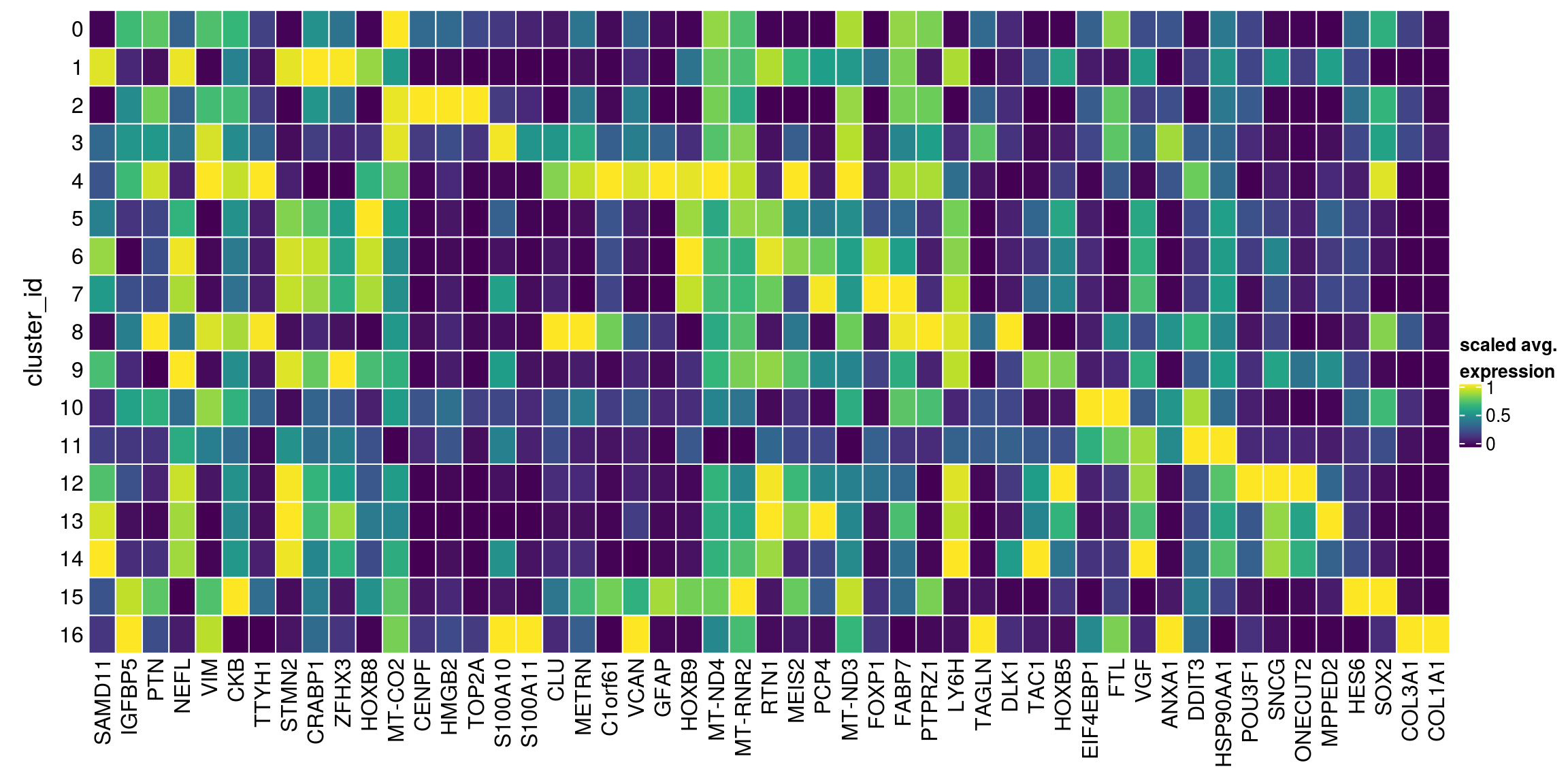
Known marker genes
## source file with list of known marker genes
source(file.path("data", "known_cell_type_markers.R"))

fs <- lapply(fs, sapply, function(g)
    grep(pattern = paste0("\\.", g, "$"), rownames(sce), value = TRUE)
  )

fs <- lapply(fs, function(x) unlist(x[lengths(x) !=0]) )

gs <- gsub(".*\\.", "", unlist(fs))
ns <- vapply(fs, length, numeric(1))
ks <- rep.int(names(fs), ns)
labs <- lapply(fs, function(x) gsub(".*\\.", "",x))
Heatmap of mean marker-exprs. by cluster
# split cells by cluster
cs_by_k <- split(colnames(sce), sce$cluster_id)
# compute cluster-marker means
ms_by_cluster <- lapply(fs, function(gs) vapply(cs_by_k, function(i)
        Matrix::rowMeans(logcounts(sce)[gs, i, drop = FALSE]),
        numeric(length(gs))))
# prep. for plotting & scale b/w 0 and 1
mat <- do.call("rbind", ms_by_cluster)
mat <- muscat:::.scale(mat)
rownames(mat) <- gs
cols <- muscat:::.cluster_colors[seq_along(fs)]
cols <- setNames(cols, names(fs))
row_anno <- rowAnnotation(
    df = data.frame(label = factor(ks, levels = names(fs))),
    col = list(label = cols), gp = gpar(col = "white"))
# percentage of cells from each of the samples per cluster
sample_props <- prop.table(n_cells, margin = 1)
col_mat <- as.matrix(unclass(sample_props))
sample_cols <- c("#882255", "#CC6677", "#11588A", "#88CCEE", "#117733", "#44AA99")
sample_cols <- setNames(sample_cols, colnames(col_mat))
col_anno <- HeatmapAnnotation(
    perc_sample = anno_barplot(col_mat, gp = gpar(fill = sample_cols),
                               height = unit(2, "cm"),
                               border = FALSE),
    annotation_label = "fraction of sample\nin cluster",
    gap = unit(10, "points"))
col_lgd <- Legend(labels = names(sample_cols),
       title = "sample",
       legend_gp = gpar(fill = sample_cols))

hm <- Heatmap(mat,
    name = "scaled avg.\nexpression",
    col = viridis(10),
    cluster_rows = FALSE,
    cluster_columns = FALSE,
    row_names_side = "left",
    column_title = "cluster_id",
    column_title_side = "bottom",
    column_names_side = "bottom",
    column_names_rot = 0,
    column_names_centered = TRUE,
    rect_gp = gpar(col = "white"),
    left_annotation = row_anno,
    top_annotation = col_anno)
draw(hm, annotation_legend_list = list(col_lgd))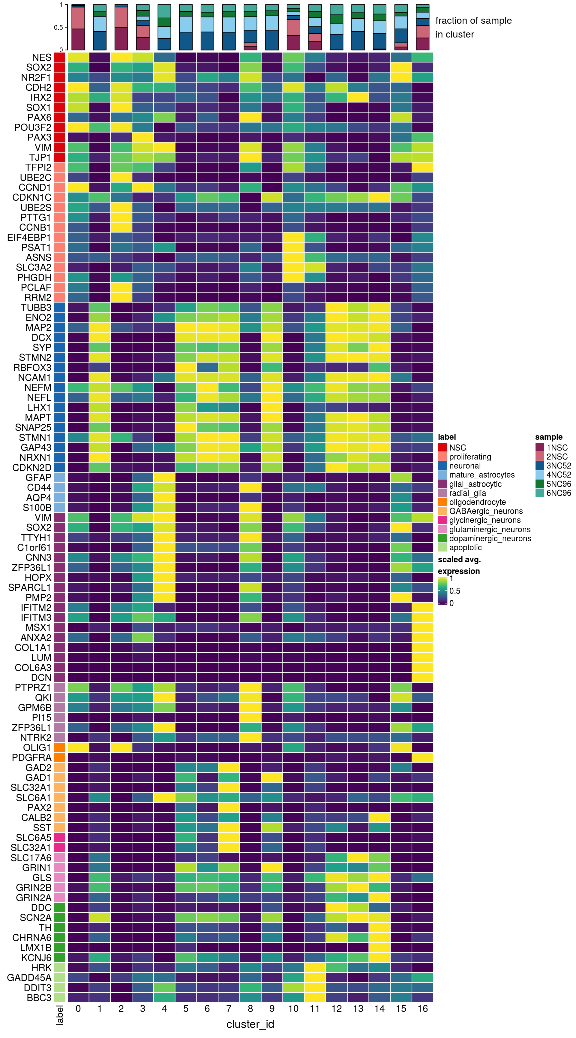
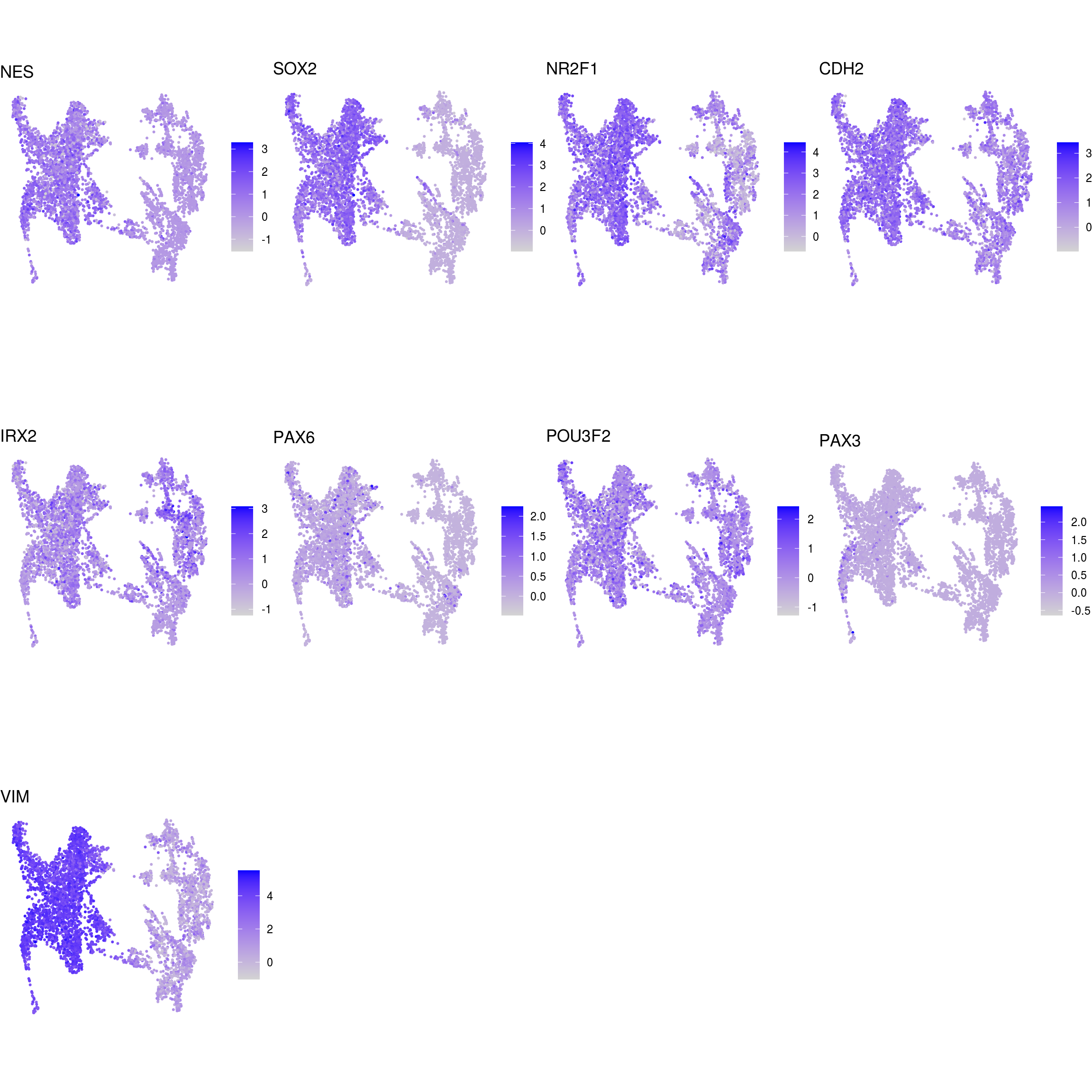
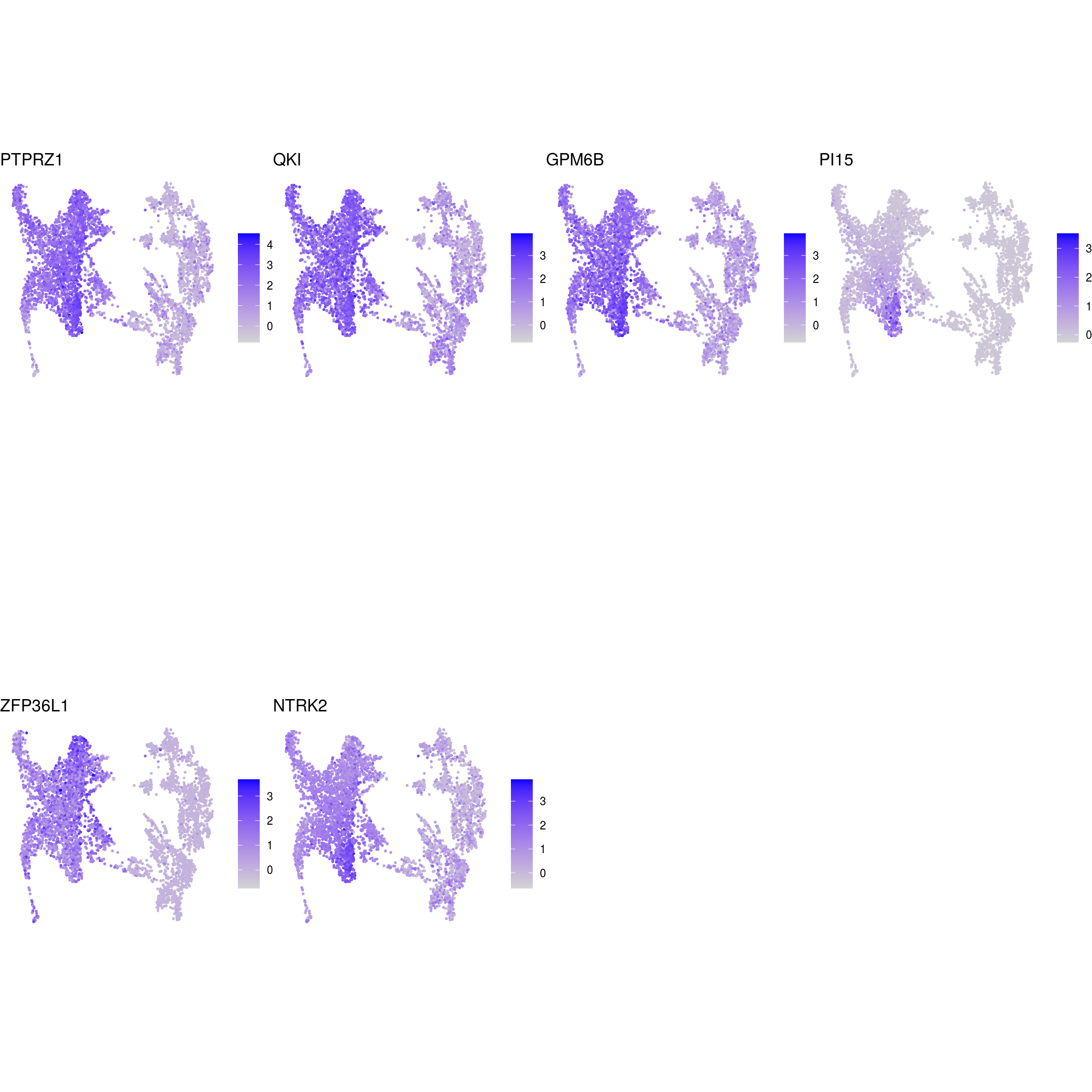
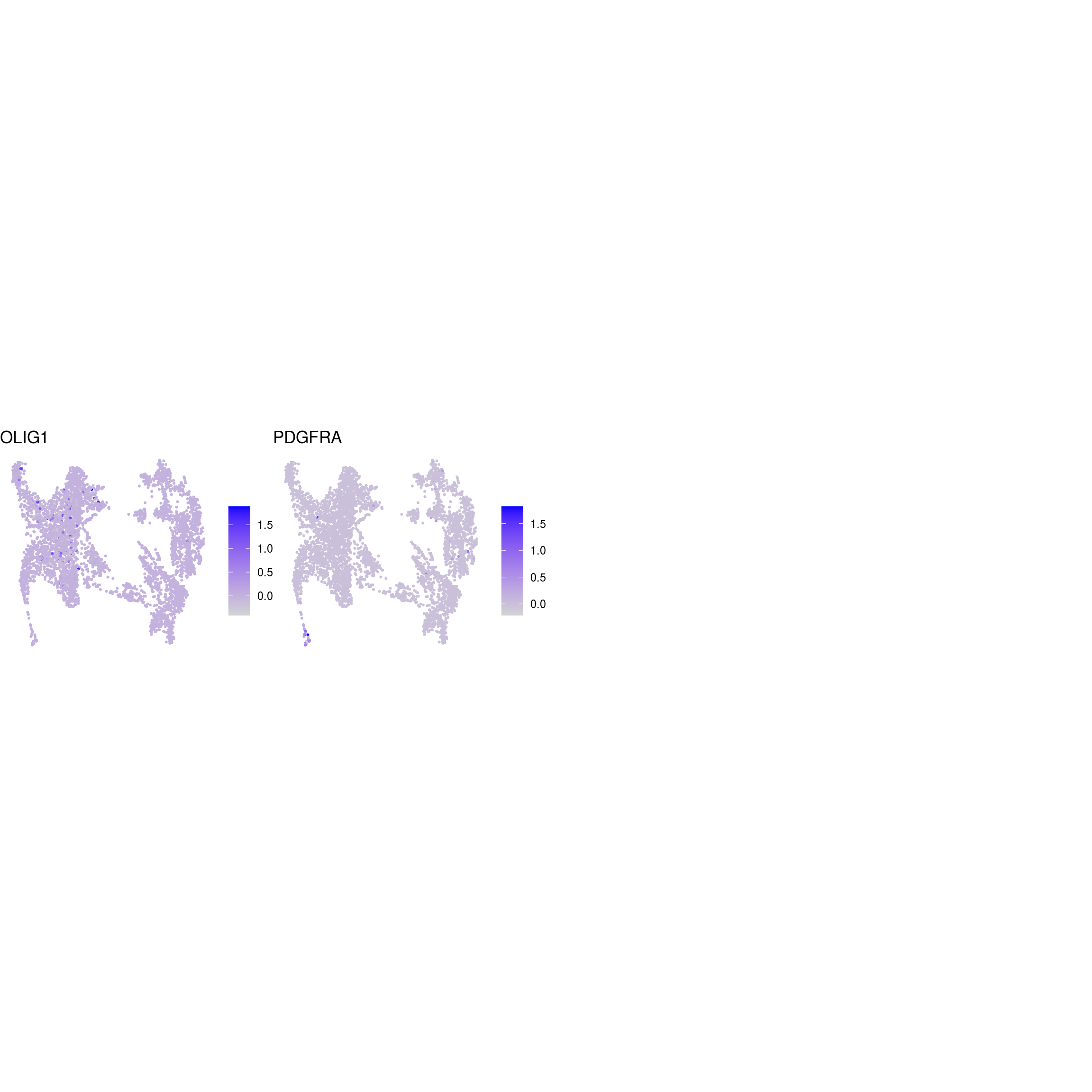
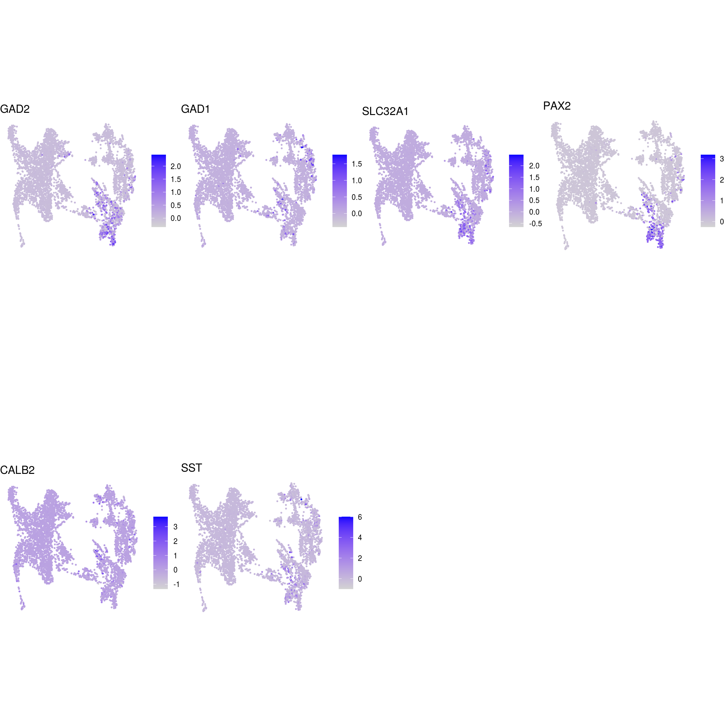
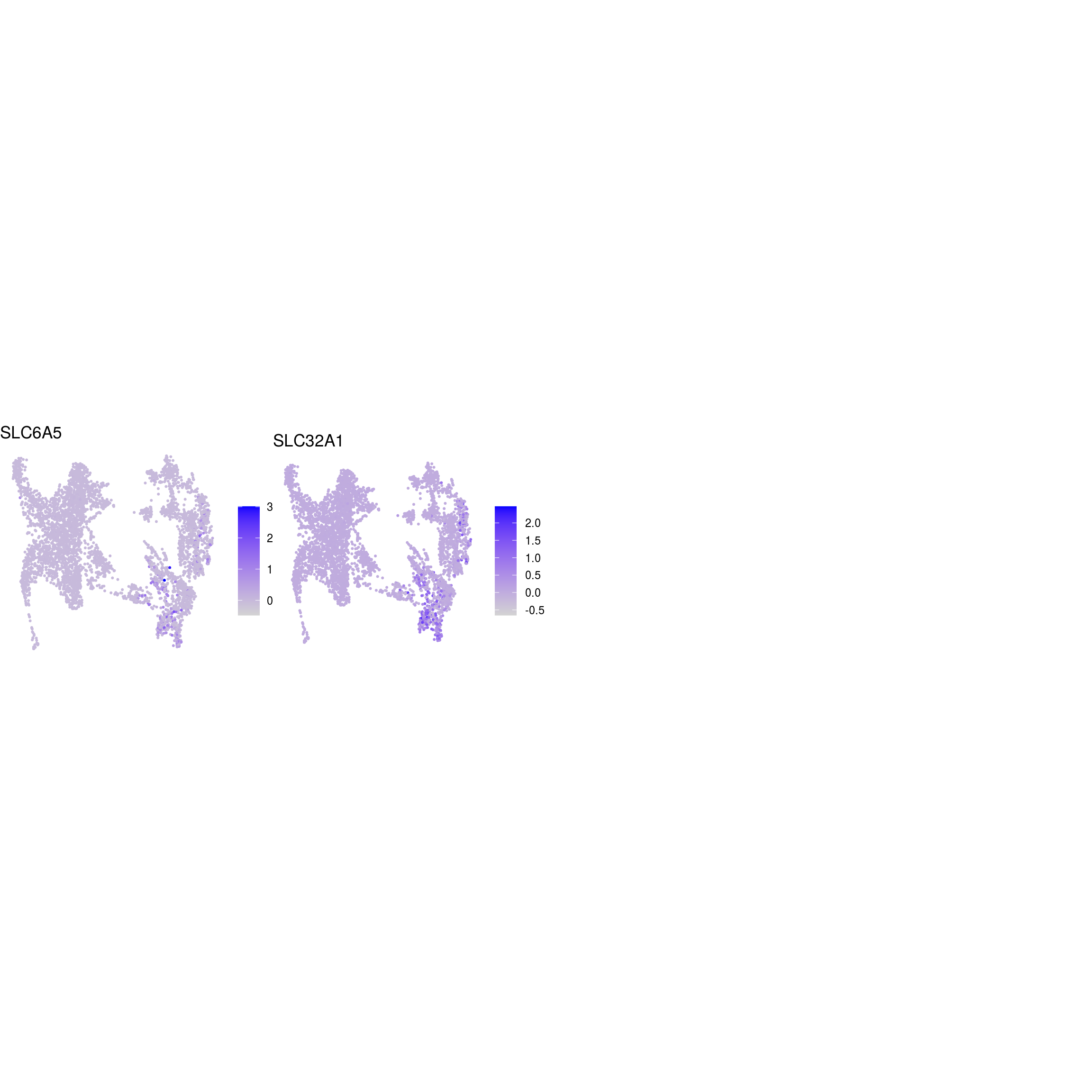
DR colored by marker expression
# downsample to 5000 cells
cs <- sample(colnames(sce), 5e3)
sub <- subset(so, cells = cs)
# UMAPs colored by marker-expression
for (m in seq_along(fs)) {
    cat("## ", names(fs)[m], "\n")
    ps <- lapply(seq_along(fs[[m]]), function(i) {
        if (!fs[[m]][i] %in% rownames(so)) return(NULL)
        FeaturePlot(sub, features = fs[[m]][i], reduction = "umap", pt.size = 0.4) +
            theme(aspect.ratio = 1, legend.position = "none") +
            ggtitle(labs[[m]][i]) + theme_void() + theme(aspect.ratio = 1)
    })
    # arrange plots in grid
    ps <- ps[!vapply(ps, is.null, logical(1))]
    p <- plot_grid(plotlist = ps, ncol = 4, label_size = 10)
    print(p)
    cat("\n\n")
}
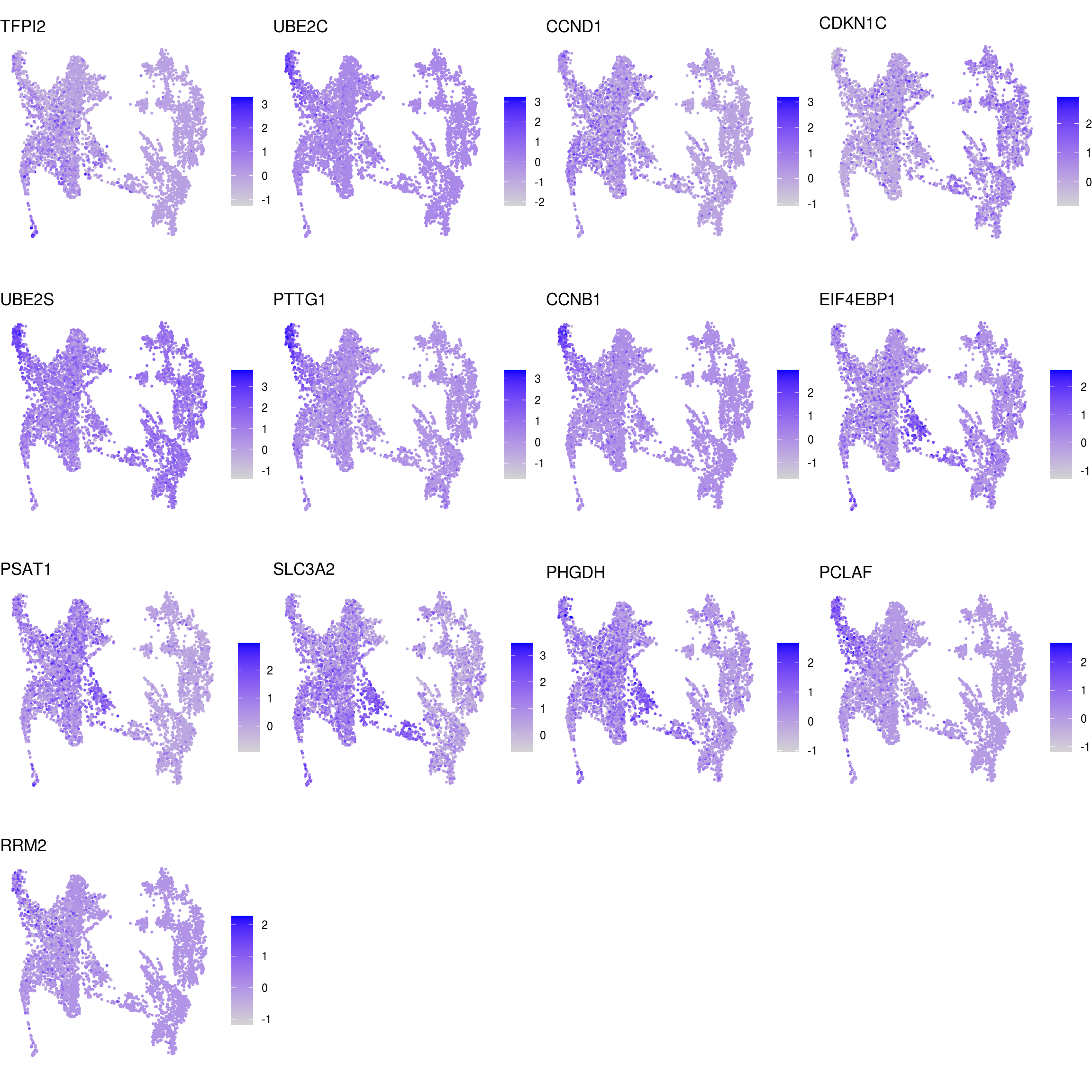
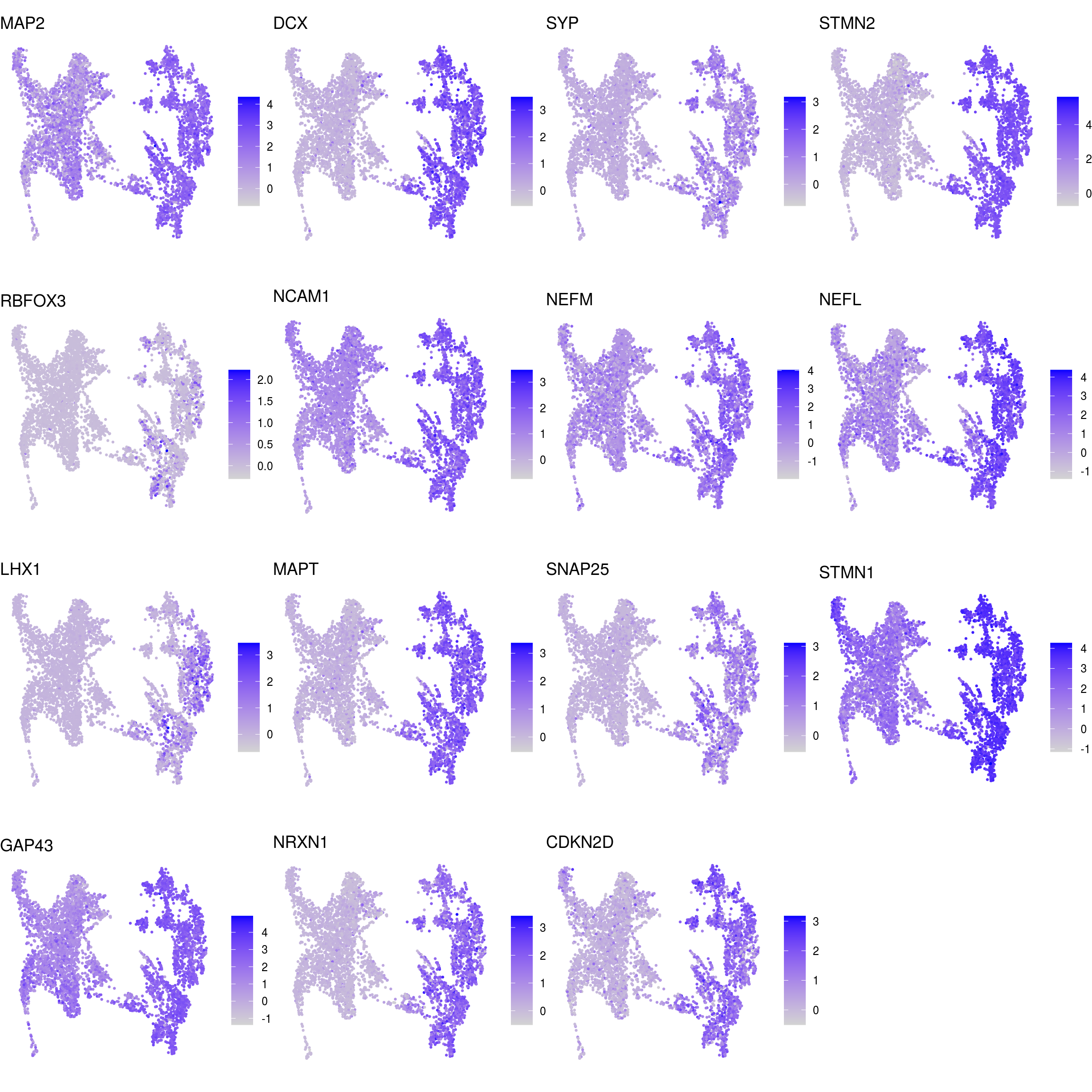
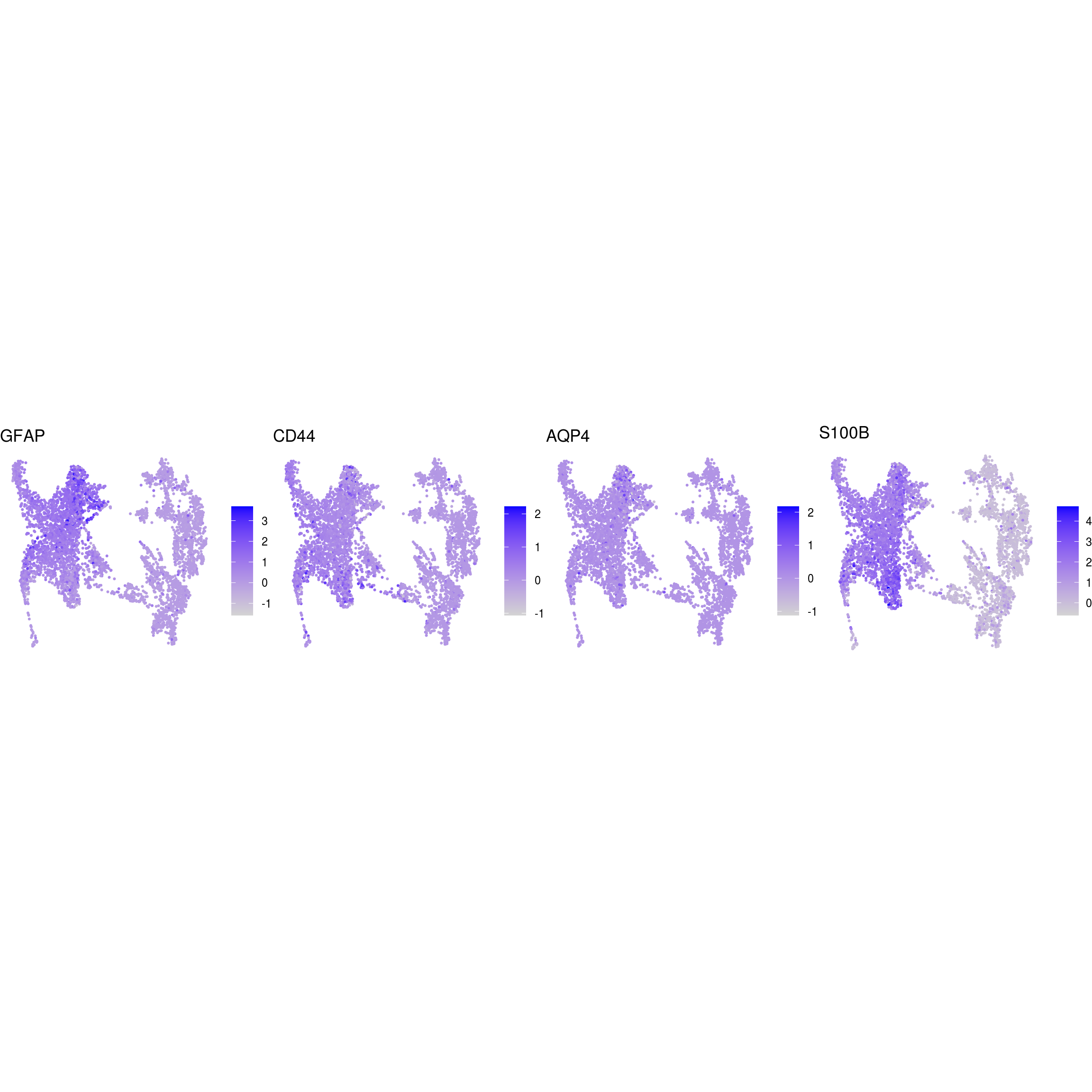
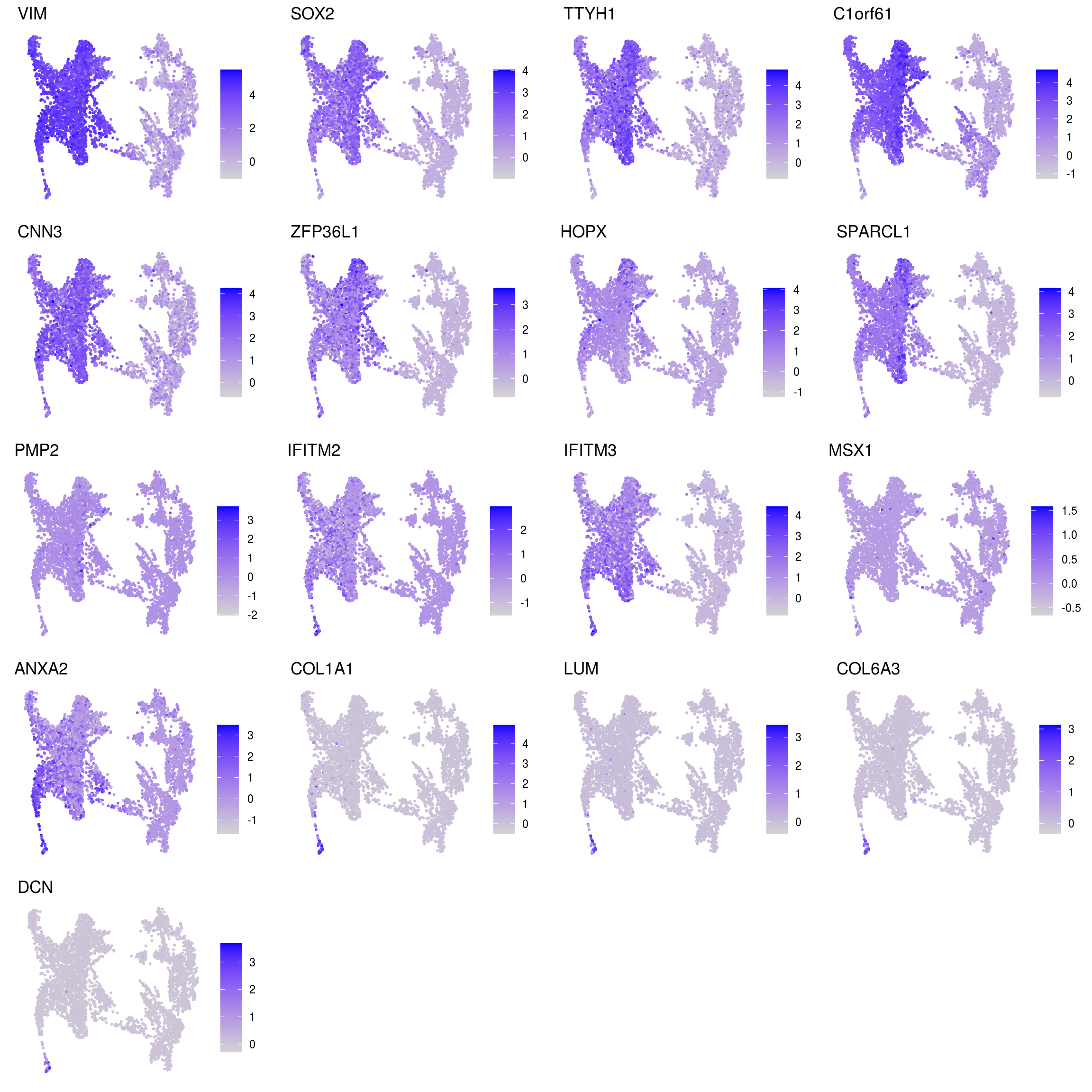
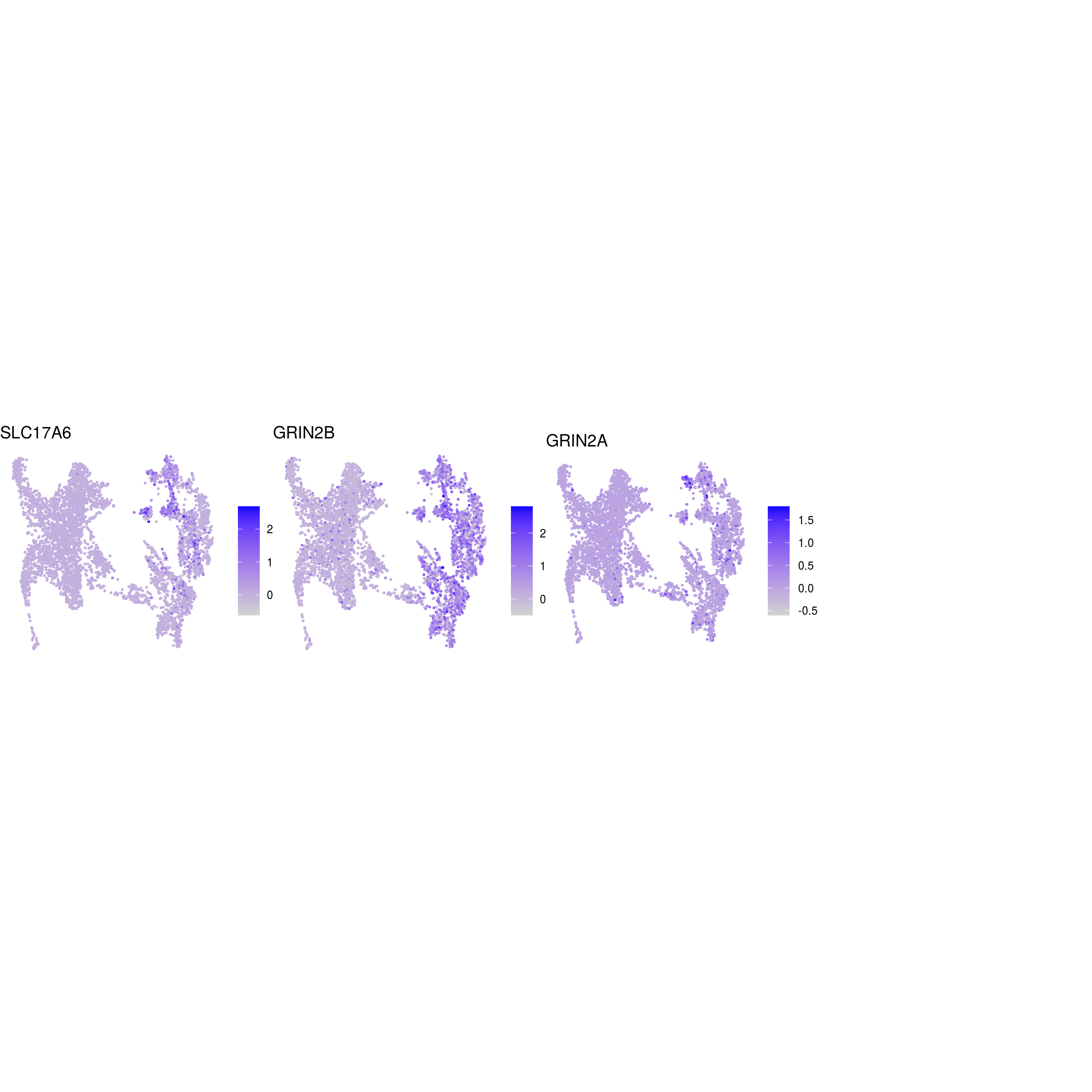
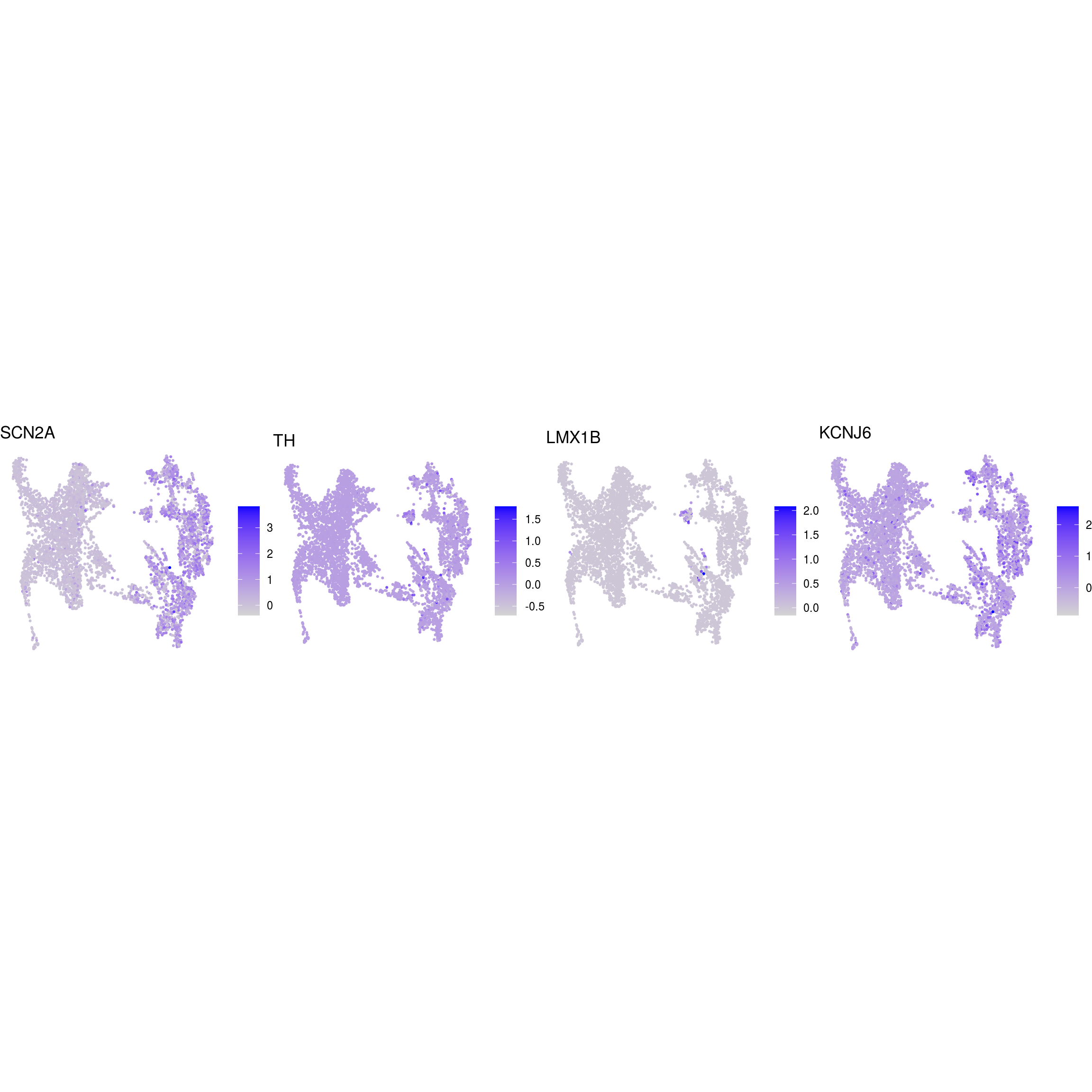
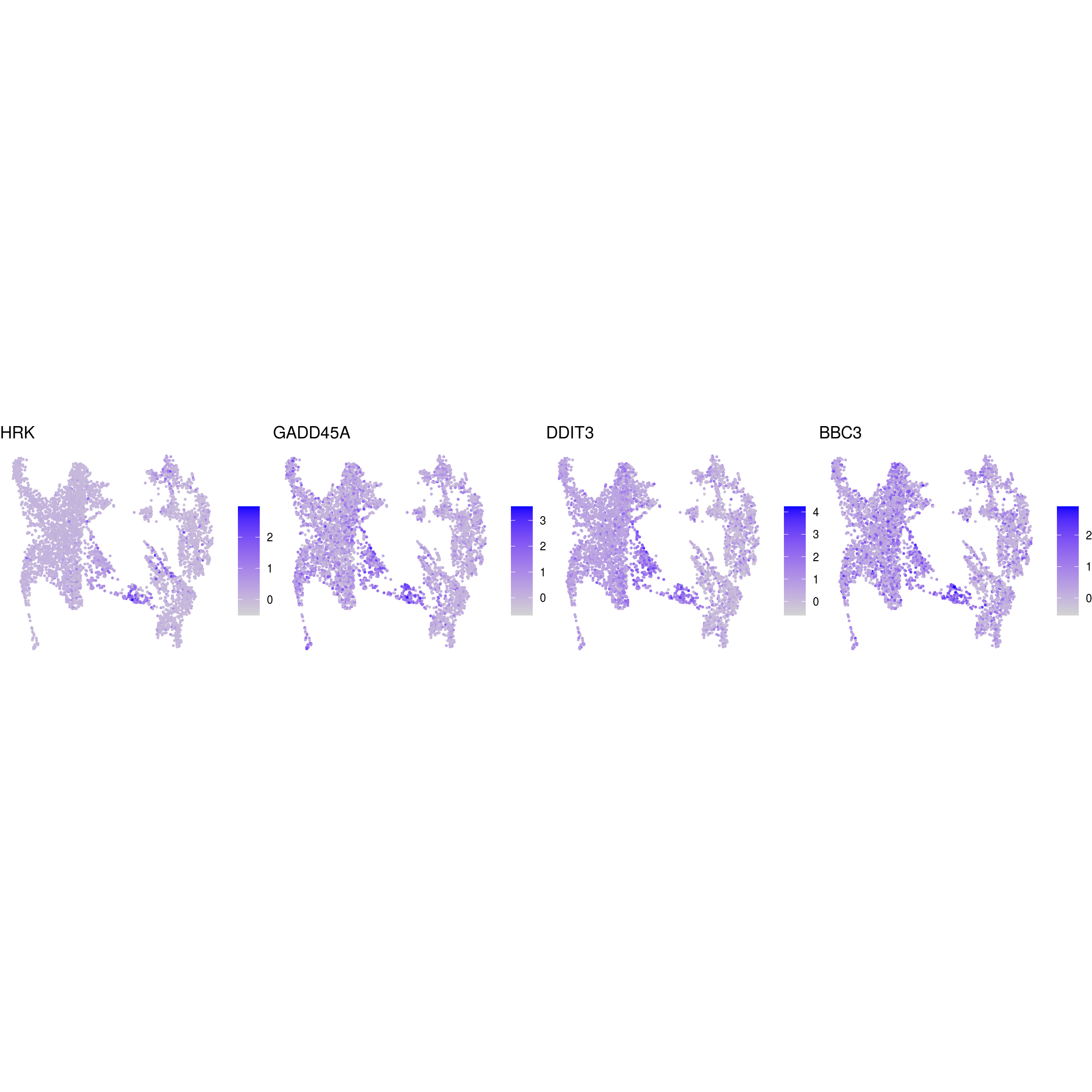
Cluster annotation
Based on the plots we annotated the clusters: …
sessionInfo()R version 4.0.0 (2020-04-24)
Platform: x86_64-pc-linux-gnu (64-bit)
Running under: Ubuntu 16.04.6 LTS
Matrix products: default
BLAS: /usr/local/R/R-4.0.0/lib/libRblas.so
LAPACK: /usr/local/R/R-4.0.0/lib/libRlapack.so
locale:
[1] LC_CTYPE=en_US.UTF-8 LC_NUMERIC=C
[3] LC_TIME=en_US.UTF-8 LC_COLLATE=en_US.UTF-8
[5] LC_MONETARY=en_US.UTF-8 LC_MESSAGES=en_US.UTF-8
[7] LC_PAPER=en_US.UTF-8 LC_NAME=C
[9] LC_ADDRESS=C LC_TELEPHONE=C
[11] LC_MEASUREMENT=en_US.UTF-8 LC_IDENTIFICATION=C
attached base packages:
[1] parallel stats4 grid stats graphics grDevices utils
[8] datasets methods base
other attached packages:
[1] BiocParallel_1.22.0 RCurl_1.98-1.2
[3] stringr_1.4.0 Seurat_3.1.5
[5] scran_1.16.0 SingleCellExperiment_1.10.1
[7] SummarizedExperiment_1.18.1 DelayedArray_0.14.0
[9] matrixStats_0.56.0 Biobase_2.48.0
[11] GenomicRanges_1.40.0 GenomeInfoDb_1.24.0
[13] IRanges_2.22.2 S4Vectors_0.26.1
[15] BiocGenerics_0.34.0 viridis_0.5.1
[17] viridisLite_0.3.0 RColorBrewer_1.1-2
[19] purrr_0.3.4 muscat_1.2.0
[21] dplyr_0.8.5 ggplot2_3.3.0
[23] cowplot_1.0.0 ComplexHeatmap_2.4.2
[25] workflowr_1.6.2
loaded via a namespace (and not attached):
[1] backports_1.1.7 circlize_0.4.9
[3] blme_1.0-4 igraph_1.2.5
[5] plyr_1.8.6 lazyeval_0.2.2
[7] TMB_1.7.16 splines_4.0.0
[9] listenv_0.8.0 scater_1.16.0
[11] digest_0.6.25 foreach_1.5.0
[13] htmltools_0.4.0 gdata_2.18.0
[15] lmerTest_3.1-2 magrittr_1.5
[17] memoise_1.1.0 cluster_2.1.0
[19] doParallel_1.0.15 ROCR_1.0-11
[21] limma_3.44.1 globals_0.12.5
[23] annotate_1.66.0 prettyunits_1.1.1
[25] colorspace_1.4-1 rappdirs_0.3.1
[27] ggrepel_0.8.2 blob_1.2.1
[29] xfun_0.14 jsonlite_1.6.1
[31] crayon_1.3.4 genefilter_1.70.0
[33] lme4_1.1-23 zoo_1.8-8
[35] ape_5.3 survival_3.1-12
[37] iterators_1.0.12 glue_1.4.1
[39] gtable_0.3.0 zlibbioc_1.34.0
[41] XVector_0.28.0 leiden_0.3.3
[43] GetoptLong_0.1.8 BiocSingular_1.4.0
[45] future.apply_1.5.0 shape_1.4.4
[47] scales_1.1.1 DBI_1.1.0
[49] edgeR_3.30.0 Rcpp_1.0.4.6
[51] xtable_1.8-4 progress_1.2.2
[53] clue_0.3-57 reticulate_1.16
[55] dqrng_0.2.1 bit_1.1-15.2
[57] rsvd_1.0.3 tsne_0.1-3
[59] htmlwidgets_1.5.1 httr_1.4.1
[61] gplots_3.0.3 ellipsis_0.3.1
[63] ica_1.0-2 farver_2.0.3
[65] pkgconfig_2.0.3 XML_3.99-0.3
[67] uwot_0.1.8 locfit_1.5-9.4
[69] labeling_0.3 tidyselect_1.1.0
[71] rlang_0.4.6 reshape2_1.4.4
[73] later_1.0.0 AnnotationDbi_1.50.0
[75] munsell_0.5.0 tools_4.0.0
[77] RSQLite_2.2.0 ggridges_0.5.2
[79] evaluate_0.14 yaml_2.2.1
[81] knitr_1.28 bit64_0.9-7
[83] fs_1.4.1 fitdistrplus_1.1-1
[85] caTools_1.18.0 RANN_2.6.1
[87] pbapply_1.4-2 future_1.17.0
[89] nlme_3.1-148 whisker_0.4
[91] pbkrtest_0.4-8.6 compiler_4.0.0
[93] plotly_4.9.2.1 beeswarm_0.2.3
[95] png_0.1-7 variancePartition_1.18.0
[97] tibble_3.0.1 statmod_1.4.34
[99] geneplotter_1.66.0 stringi_1.4.6
[101] lattice_0.20-41 Matrix_1.2-18
[103] nloptr_1.2.2.1 vctrs_0.3.0
[105] pillar_1.4.4 lifecycle_0.2.0
[107] lmtest_0.9-37 GlobalOptions_0.1.1
[109] RcppAnnoy_0.0.16 BiocNeighbors_1.6.0
[111] data.table_1.12.8 bitops_1.0-6
[113] irlba_2.3.3 patchwork_1.0.0
[115] httpuv_1.5.2 colorRamps_2.3
[117] R6_2.4.1 promises_1.1.0
[119] KernSmooth_2.23-17 gridExtra_2.3
[121] vipor_0.4.5 codetools_0.2-16
[123] boot_1.3-25 MASS_7.3-51.6
[125] gtools_3.8.2 assertthat_0.2.1
[127] DESeq2_1.28.1 rprojroot_1.3-2
[129] rjson_0.2.20 withr_2.2.0
[131] sctransform_0.2.1 GenomeInfoDbData_1.2.3
[133] hms_0.5.3 tidyr_1.1.0
[135] glmmTMB_1.0.1 minqa_1.2.4
[137] rmarkdown_2.1 DelayedMatrixStats_1.10.0
[139] Rtsne_0.15 git2r_0.27.1
[141] numDeriv_2016.8-1.1 ggbeeswarm_0.6.0