Quality control with SampleQC
Katharina Hembach
June 08, 2020
Last updated: 2020-06-08
Checks: 7 0
Knit directory: neural_scRNAseq/
This reproducible R Markdown analysis was created with workflowr (version 1.6.2). The Checks tab describes the reproducibility checks that were applied when the results were created. The Past versions tab lists the development history.
Great! Since the R Markdown file has been committed to the Git repository, you know the exact version of the code that produced these results.
Great job! The global environment was empty. Objects defined in the global environment can affect the analysis in your R Markdown file in unknown ways. For reproduciblity it’s best to always run the code in an empty environment.
The command set.seed(20200522) was run prior to running the code in the R Markdown file. Setting a seed ensures that any results that rely on randomness, e.g. subsampling or permutations, are reproducible.
Great job! Recording the operating system, R version, and package versions is critical for reproducibility.
Nice! There were no cached chunks for this analysis, so you can be confident that you successfully produced the results during this run.
Great job! Using relative paths to the files within your workflowr project makes it easier to run your code on other machines.
Great! You are using Git for version control. Tracking code development and connecting the code version to the results is critical for reproducibility.
The results in this page were generated with repository version 013c877. See the Past versions tab to see a history of the changes made to the R Markdown and HTML files.
Note that you need to be careful to ensure that all relevant files for the analysis have been committed to Git prior to generating the results (you can use wflow_publish or wflow_git_commit). workflowr only checks the R Markdown file, but you know if there are other scripts or data files that it depends on. Below is the status of the Git repository when the results were generated:
Ignored files:
    Ignored:    .DS_Store
    Ignored:    .Rhistory
    Ignored:    .Rproj.user/
    Ignored:    ._.DS_Store
    Ignored:    .__workflowr.yml
    Ignored:    ._neural_scRNAseq.Rproj
    Ignored:    analysis/.DS_Store
    Ignored:    analysis/.Rhistory
    Ignored:    analysis/._.DS_Store
    Ignored:    analysis/._01-preprocessing.Rmd
    Ignored:    analysis/._01-preprocessing.html
    Ignored:    analysis/._02.1-SampleQC.Rmd
    Ignored:    analysis/._04-clustering.Rmd
    Ignored:    analysis/._04-clustering.knit.md
    Ignored:    analysis/.__site.yml
    Ignored:    analysis/01-preprocessing_cache/
    Ignored:    analysis/02-1-SampleQC_cache/
    Ignored:    analysis/02-quality_control_cache/
    Ignored:    analysis/03-filtering_cache/
    Ignored:    analysis/04-clustering_cache/
    Ignored:    analysis/05-annotation_cache/
    Ignored:    analysis/sample5_QC_cache/
    Ignored:    data/.DS_Store
    Ignored:    data/._.DS_Store
    Ignored:    data/._metadata.csv
    Ignored:    data/._metadata.xlsx
    Ignored:    data/.smbdeleteAAA17ed8b4b
    Ignored:    data/data_sushi/
    Ignored:    data/filtered_feature_matrices/
    Ignored:    data/metadata.csv
    Ignored:    data/metadata.xlsx
    Ignored:    output/.DS_Store
    Ignored:    output/._.DS_Store
    Ignored:    output/figures/
    Ignored:    output/sce_01_preprocessing.rds
    Ignored:    output/sce_02_quality_control.rds
    Ignored:    output/sce_03_filtering.rds
    Ignored:    output/sce_preprocessing.rds
    Ignored:    output/so_04_clustering.rds

Untracked files:
    Untracked:  analysis/sample5_QC.Rmd
    Untracked:  scripts/

Unstaged changes:
    Modified:   analysis/04-clustering.Rmd
    Modified:   analysis/_site.yml
Note that any generated files, e.g. HTML, png, CSS, etc., are not included in this status report because it is ok for generated content to have uncommitted changes.
These are the previous versions of the repository in which changes were made to the R Markdown (analysis/02.1-SampleQC.Rmd) and HTML (docs/02.1-SampleQC.html) files. If you’ve configured a remote Git repository (see ?wflow_git_remote), click on the hyperlinks in the table below to view the files as they were in that past version.
| File | Version | Author | Date | Message |
|---|---|---|---|---|
| html | 1230f08 | khembach | 2020-05-27 | Build site. |
| Rmd | 6be1a5a | khembach | 2020-05-27 | rebuild without cache and SampleQC report |
Load packages
library(SampleQC)
library(dplyr)
library(patchwork)
library(SingleCellExperiment)
Here, I am testing the SampleQC package from Will Macnair.
Load data and preparation
sce <- readRDS(file.path("output", "sce_02_quality_control.rds"))
qc_df <- colData(sce) %>% as.data.frame() %>%
  dplyr::mutate(cell_id = paste(barcode, sample_id, sep = "."),
                log_counts = log10(total), log_feats = log10(detected),
                logit_mito = qlogis( (subsets_Mt_sum + 1)/(total + 2) ) )

qc_dt <- make_qc_dt(qc_df)
Running SampleQC
# which QC metrics do we want to use? (the most important bit)
qc_names <- c('log_counts', 'log_feats', 'logit_mito')
# which discrete-valued variables do we want to annotate the samples with?
annot_discrete <- c("group_id")

## Calculate distances between all samples and run dimension reduction
mmd_list <- calculate_sample_to_sample_MMDs(qc_dt, qc_names,
                                            subsample=200, n_times=20,
                                            n_cores=20)
mmd_list <- embed_sample_to_sample_MMDs(mmd_list, qc_dt, annot_discrete,
                                        n_nhbrs=5)
print(table(mmd_list$mmd_clusts))
1
6
## We fit Gaussian mixture models to the whole dataset, because we only have
## 6 samples
em_list <- fit_sampleQC(mmd_list, qc_dt, qc_names, K_all=1)max 50 EM iterations:
.
took 1 iterationsReport setup
Following report is copied from Will’s github repository.
# define what to use and annotate
qc_names        = em_list[[1]]$qc_names
cluster_names   = names(em_list)
n_clusters      = length(em_list)
Checking for outliers and QC batches via MMD
Maximum mean discrepancy (MMD) is a measure of dissimilarity of empirical (possibly multivariate) distributions. If \(X\) and \(Y\) are sampled from distributions \(D_x\) and \(D_y\), then \(E(MMD(X,Y)) = 0\) if and only if \(D_x = D_y\). SampleQC uses MMD to estimate similarities between the QC matrices of samples in a experiment. Viewed as equivalent to a distance, SampleQC uses the MMD values as input to multiple non-linear embedding approaches, and for clustering. This then allows users to identify possible batch effects in the samples, and groupings of samples which have similar distributions of QC metrics.
Plot MMD dissimilarity matrix
Heatmap of all pairwise dissimilarities between samples (values close to 0 indicate similar samples; values of 1 and higher indicate extremely dissimilar samples).
(plot_mmd_heatmap(mmd_list))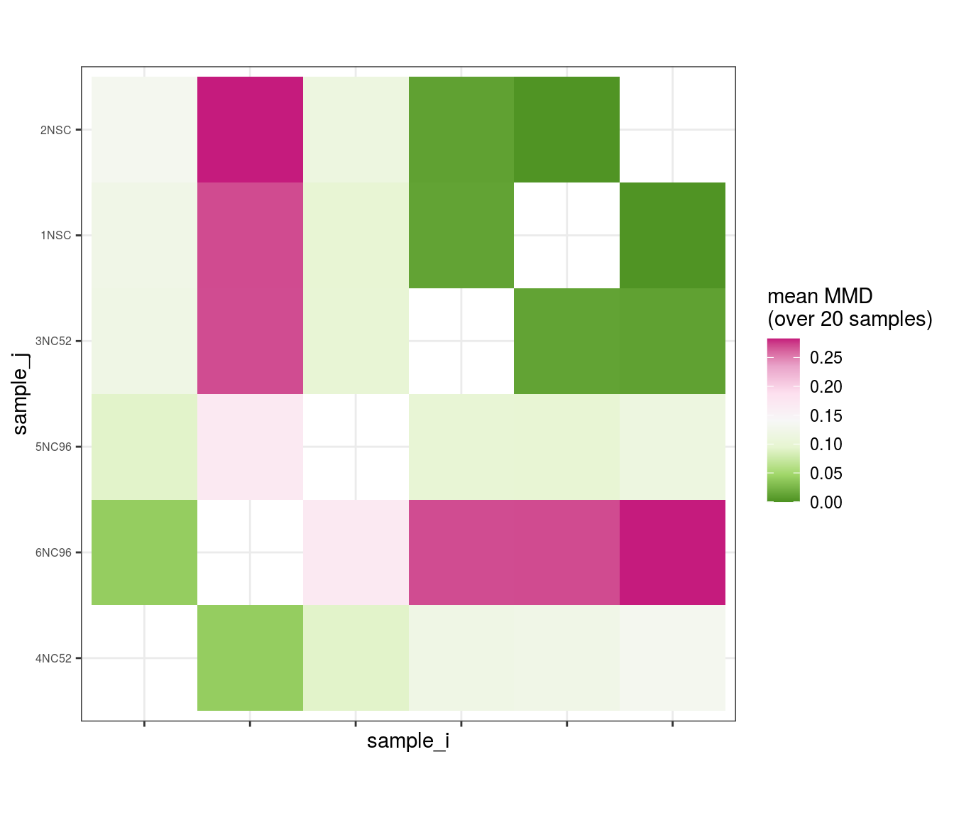
| Version | Author | Date |
|---|---|---|
| 1230f08 | khembach | 2020-05-27 |
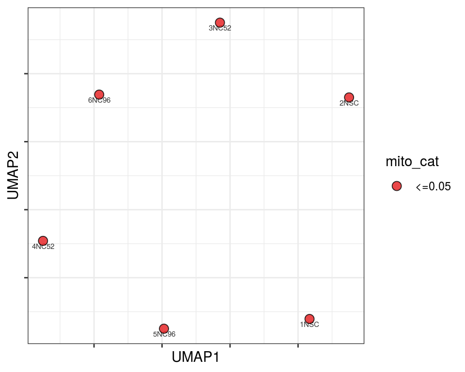
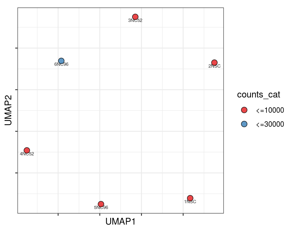
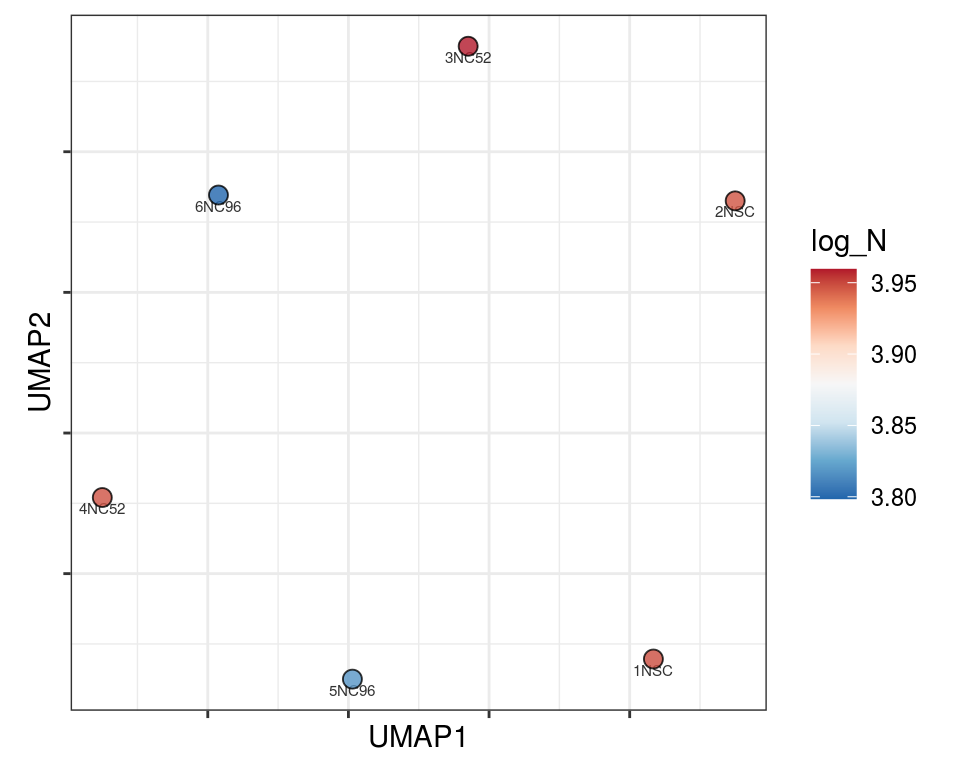
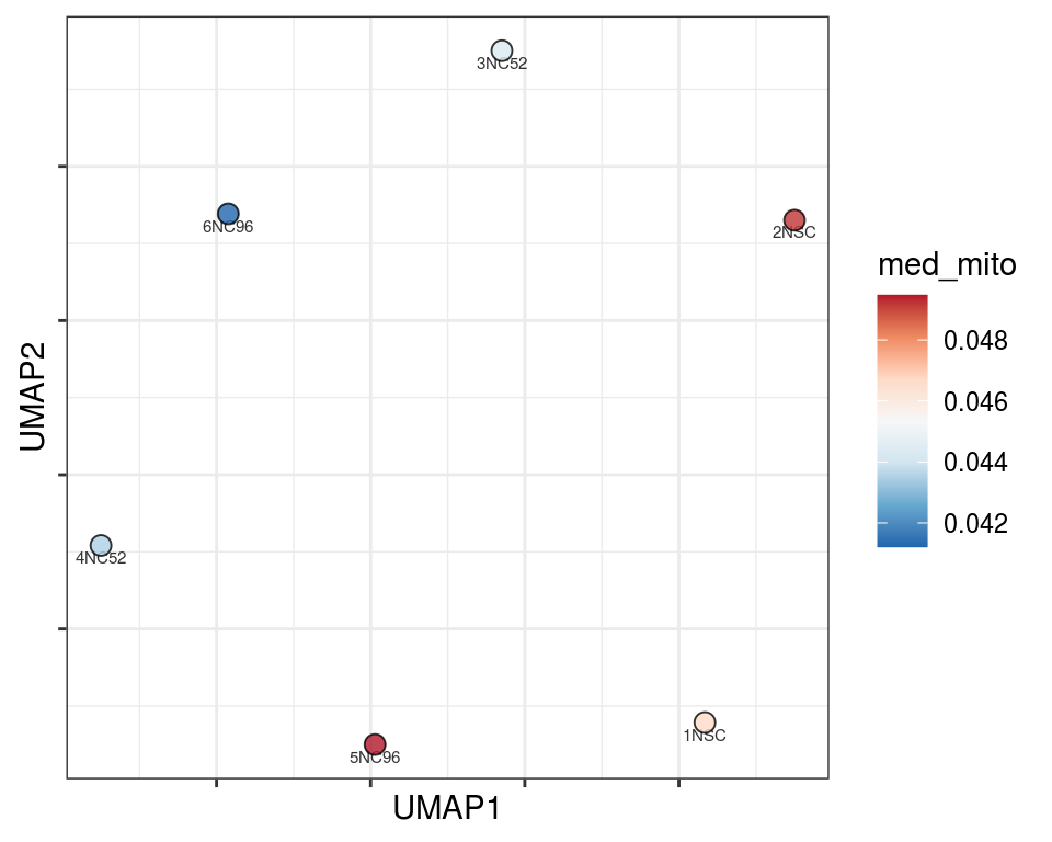
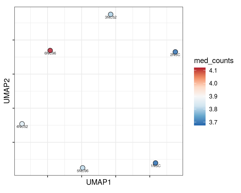
Plot over UMAP embedding with annotations
UMAP embedding of dissimilarity matrix, annotated with selected discrete and continuous values for each sample.
plot_embeddings(mmd_list, "discrete", "UMAP")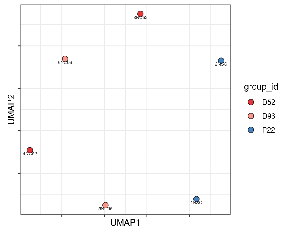
QC_clust
N_cat
Warning in brewer.pal(n_cols, "PiYG"): minimal value for n is 3, returning requested palette with 3 different levels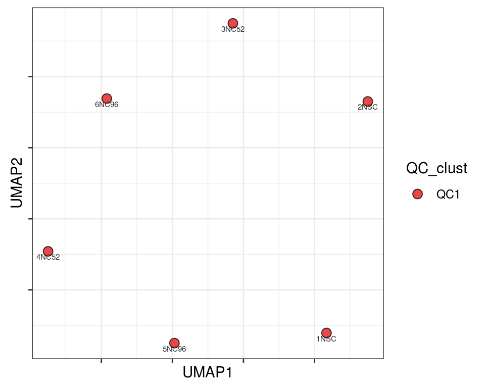
| Version | Author | Date |
|---|---|---|
| 1230f08 | khembach | 2020-05-27 |
mito_cat
Warning in brewer.pal(n_cols, "PiYG"): minimal value for n is 3, returning requested palette with 3 different levels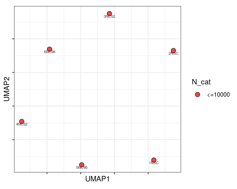
| Version | Author | Date |
|---|---|---|
| 1230f08 | khembach | 2020-05-27 |
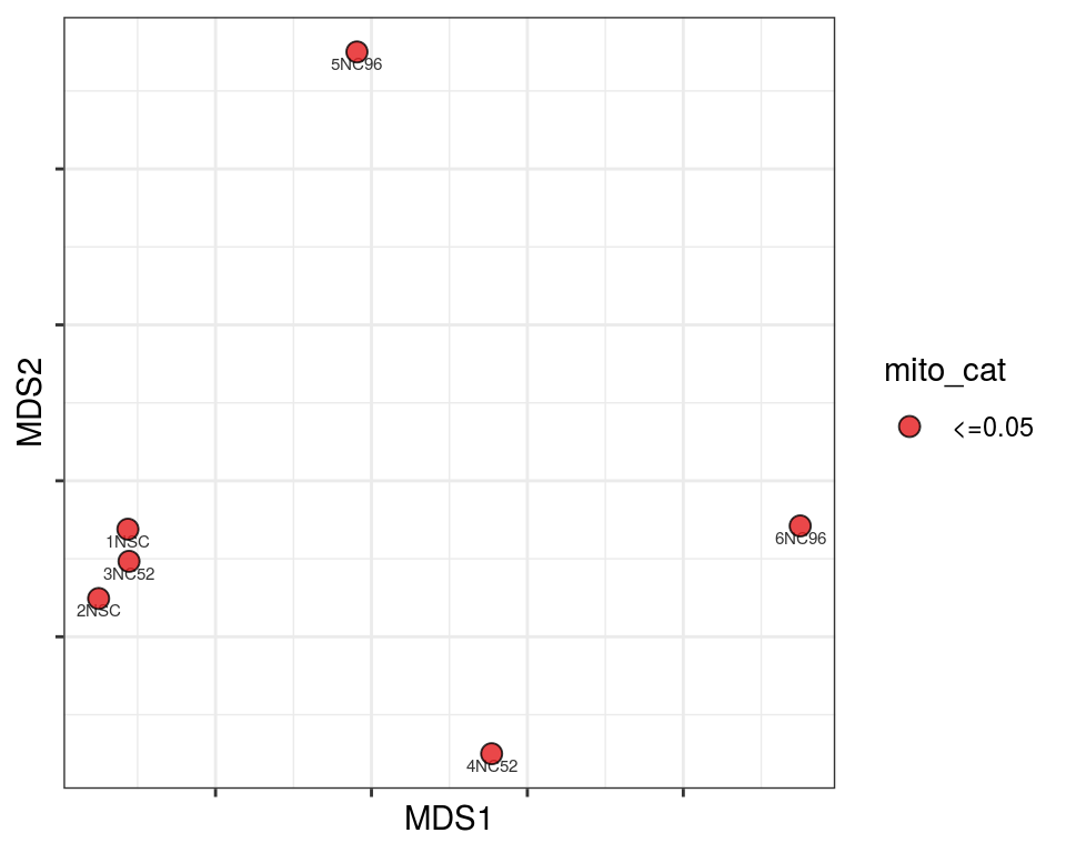
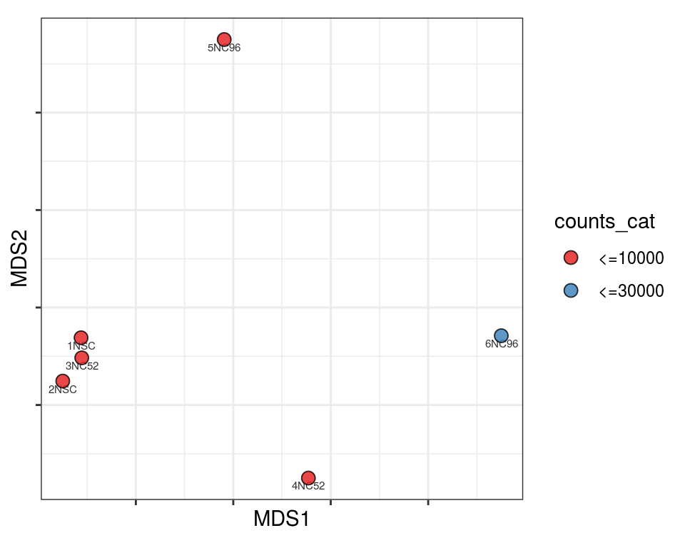
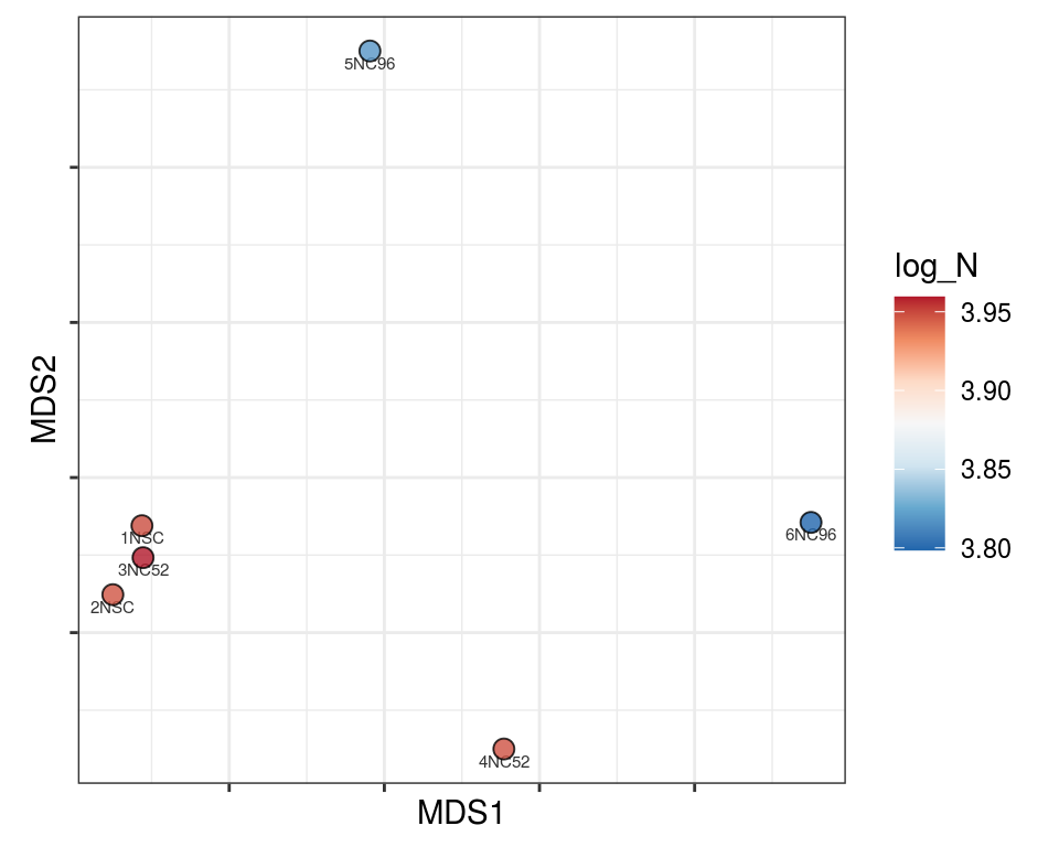
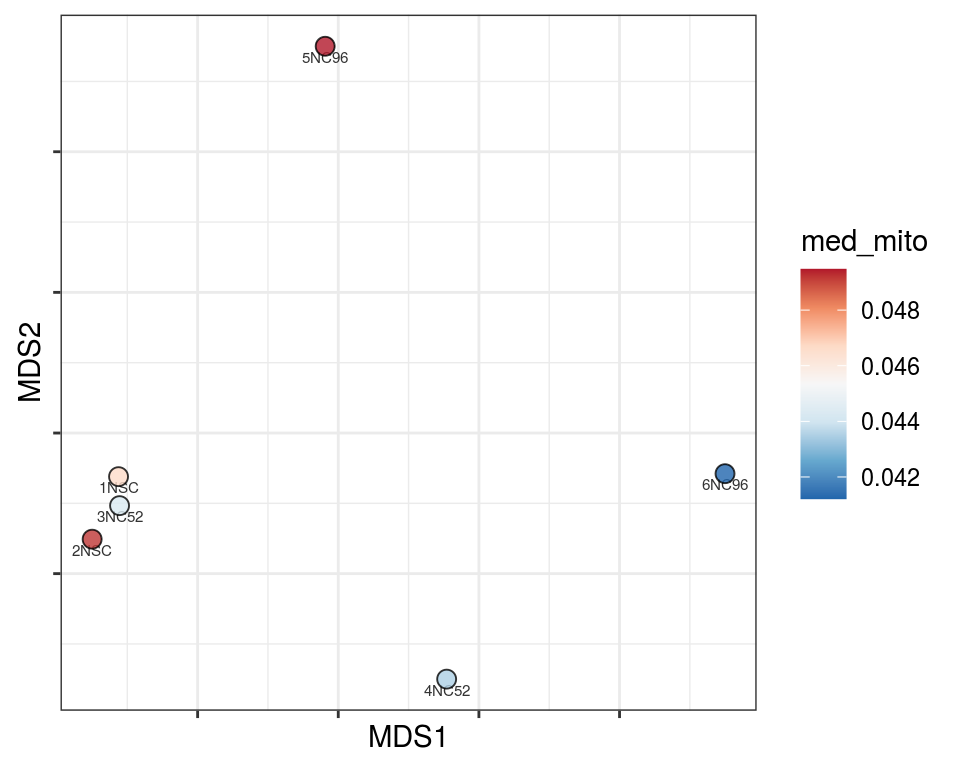
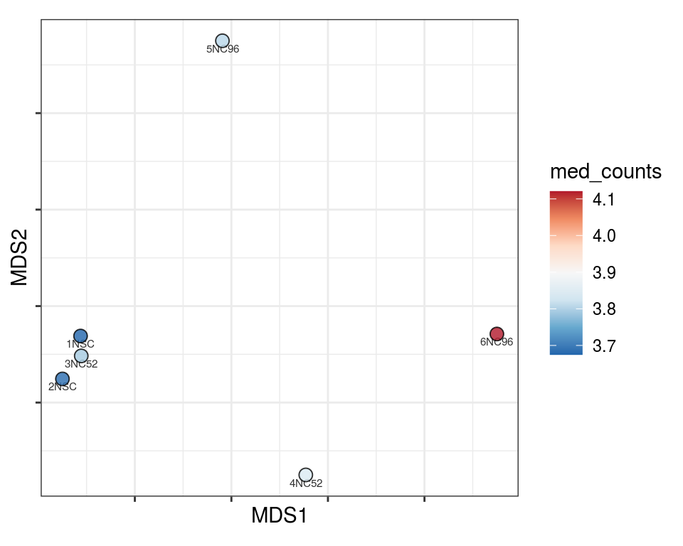
Plot over MDS embedding with annotations
Multidimensional scaling (MDS) embedding of dissimilarity matrix, annotated with selected discrete and continuous values for each sample.
plot_embeddings(mmd_list, "discrete", "MDS")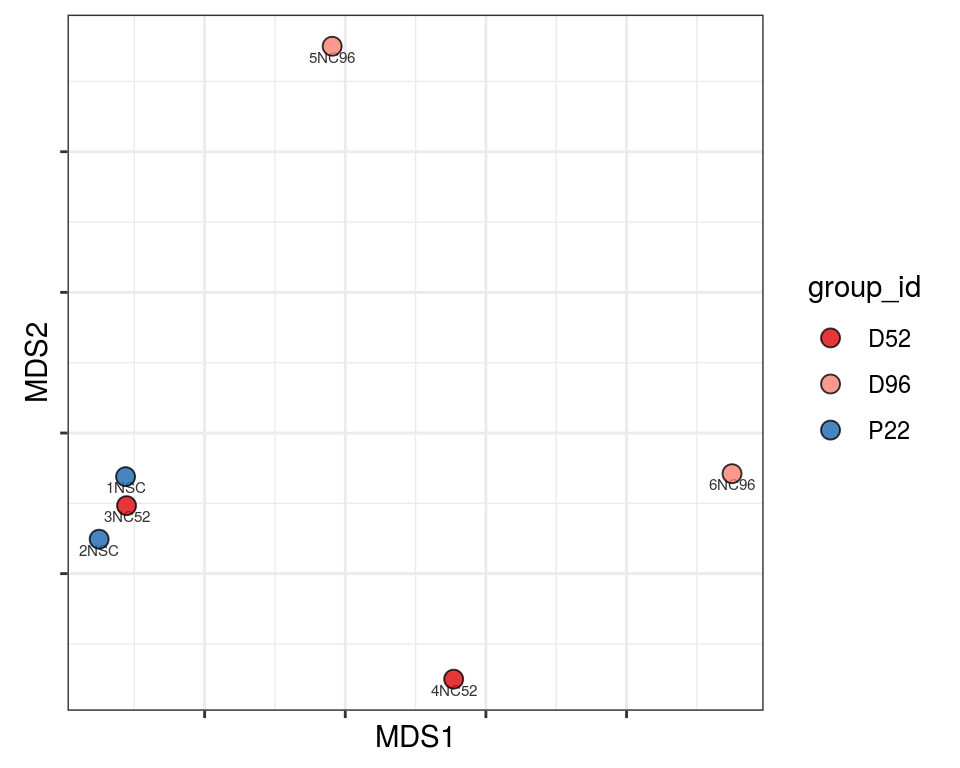
QC_clust
N_cat
Warning in brewer.pal(n_cols, "PiYG"): minimal value for n is 3, returning requested palette with 3 different levels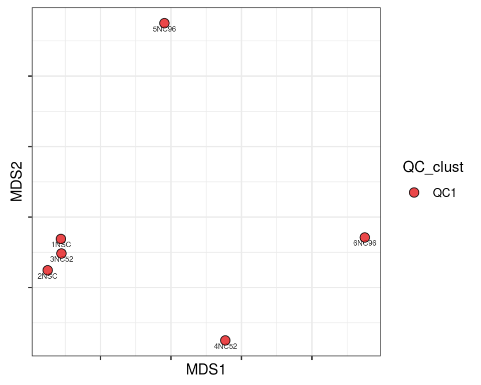
| Version | Author | Date |
|---|---|---|
| 1230f08 | khembach | 2020-05-27 |
mito_cat
Warning in brewer.pal(n_cols, "PiYG"): minimal value for n is 3, returning requested palette with 3 different levels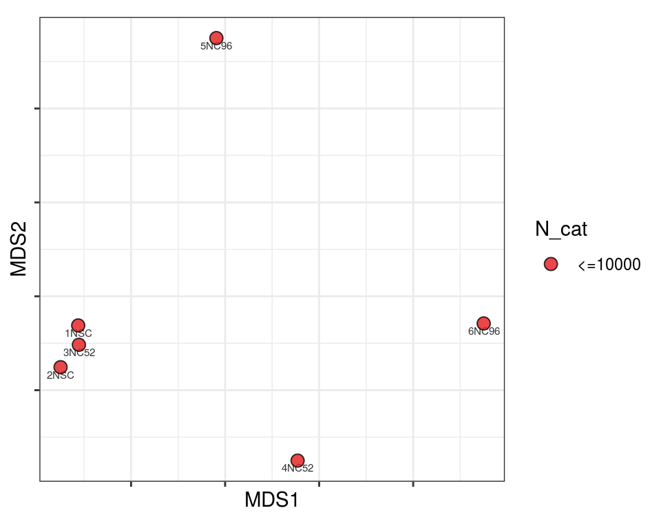
| Version | Author | Date |
|---|---|---|
| 1230f08 | khembach | 2020-05-27 |
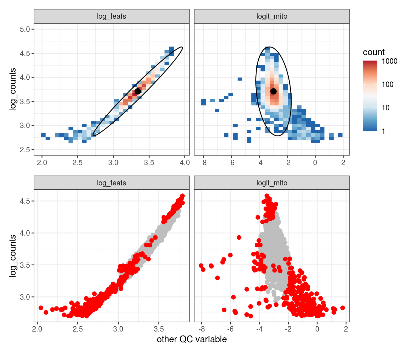
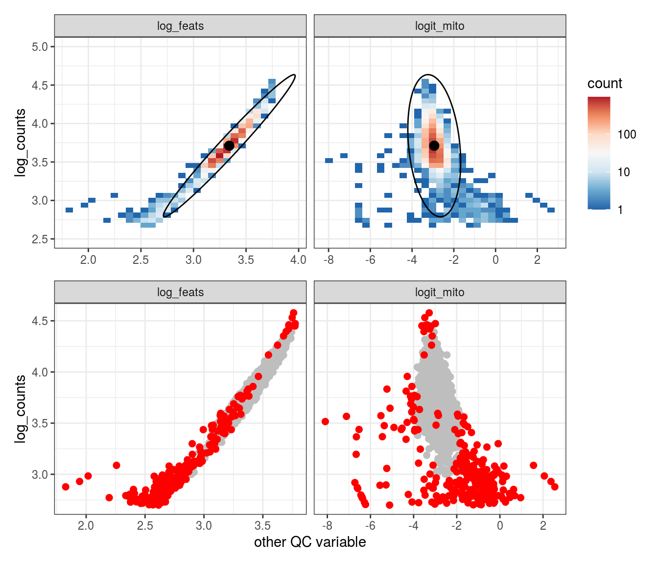
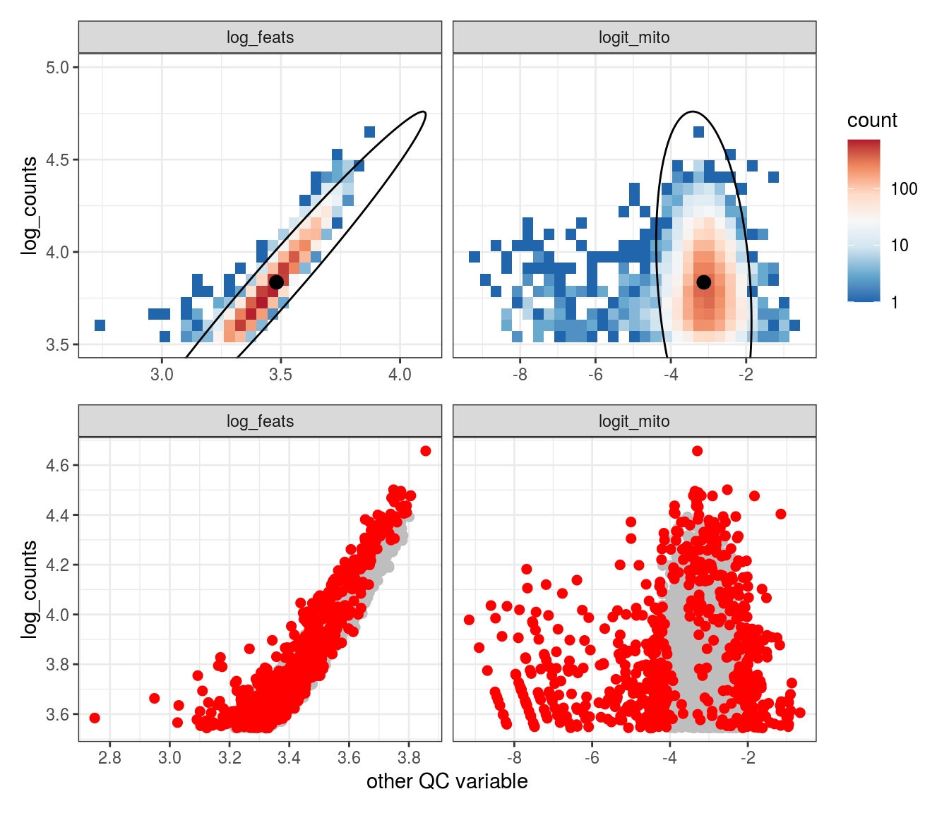
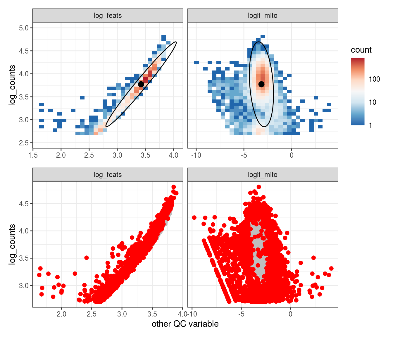
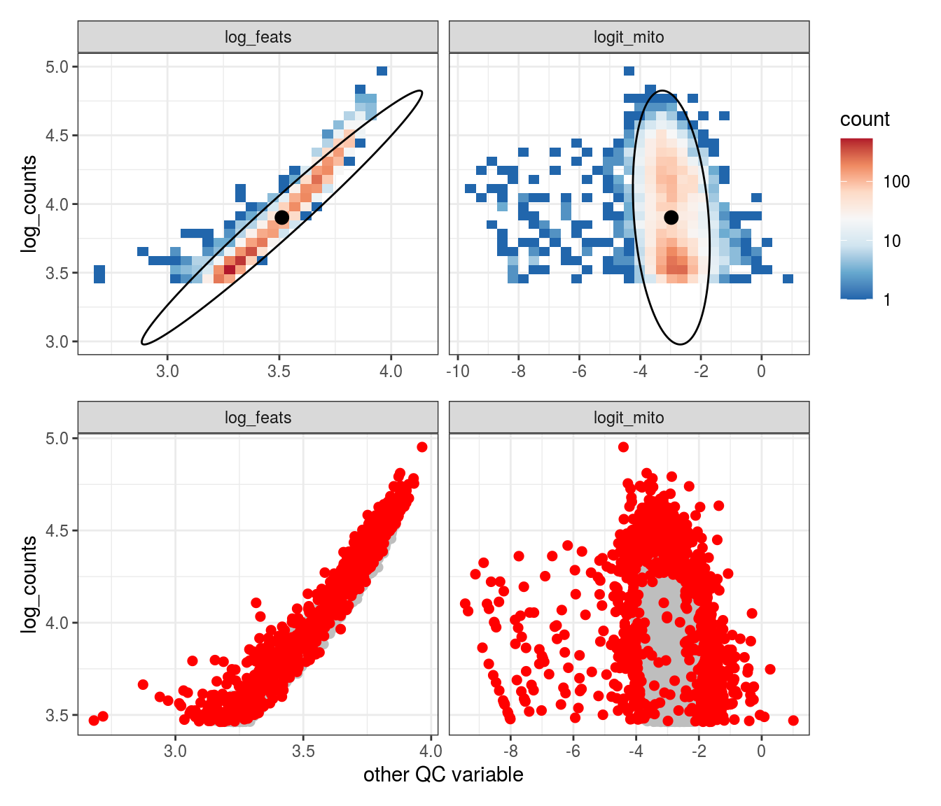
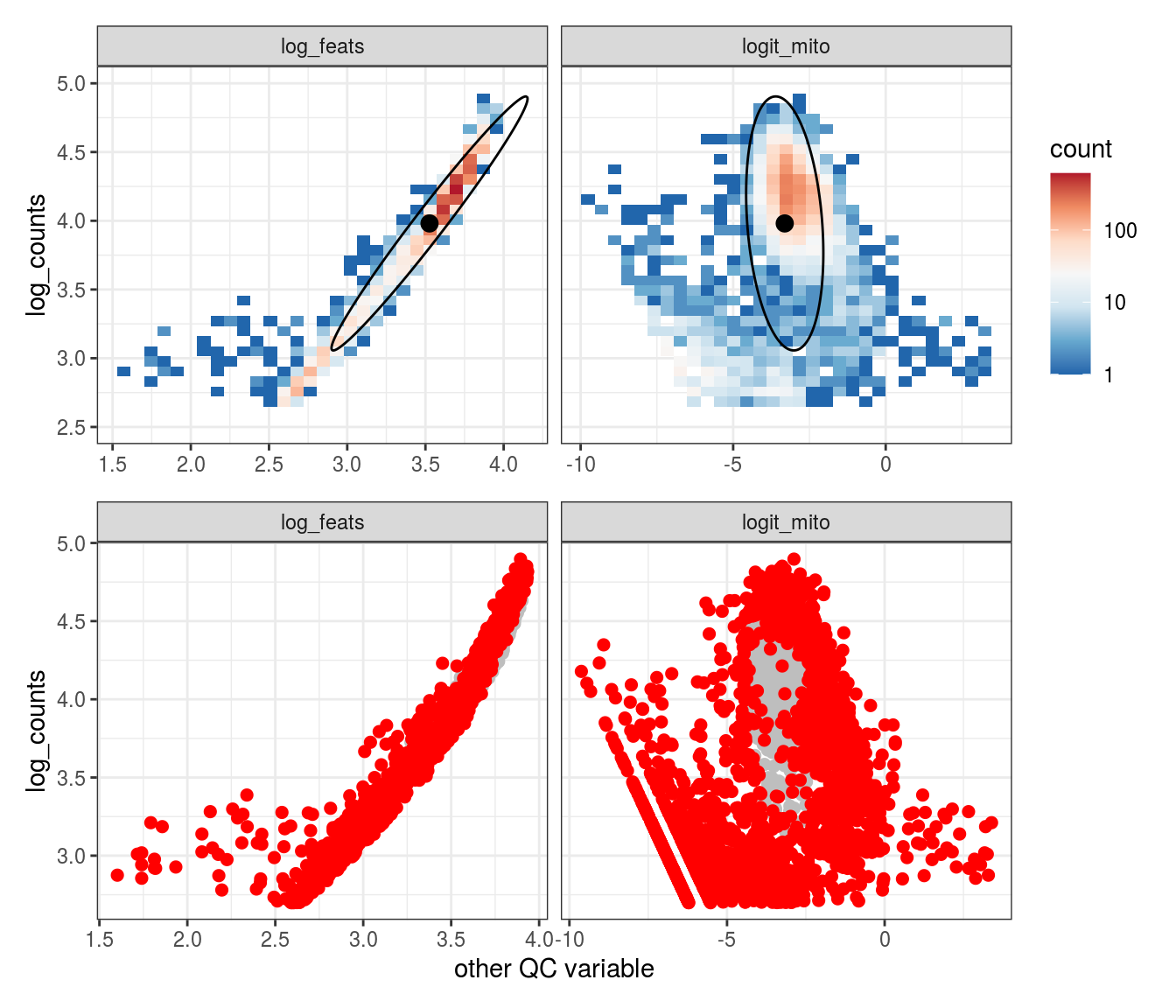
Plot SampleQC model fits and outliers over QC biaxials
These plots show biaxial distributions of each sample, annotated with both the fitted mean and covariance matrices, and the cells which are then identified as outliers. You can use this to check that you have the correct number of components for each sample grouping, and to check that the fitting procedure has worked properly. The means and covariances of the components should match up to the densest parts of the biaxial plots.
alpha_cut   = 0.001
for (ii in 1:n_clusters) {
    cat('## ', cluster_names[ii], '{.tabset}\n')
    for (s in sort(em_list[[ii]]$sample_list)) {
        cat('### ', s, ' \n')
        g_fit   = plot_fit_over_biaxials_one_sample(em_list[[ii]], qc_dt, s, qc_names, alpha_cut)
        g_out   = plot_outliers_one_sample(em_list[[ii]], s)
        g       = g_fit / g_out
        print(g)
        cat('\n\n')
    }
}
All
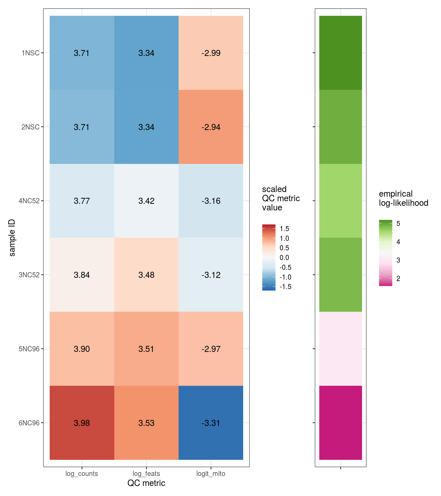
Plot parameters
These plots show the fitted parameters for each sample and each mixture component. There are two sets of parameters: \(\alpha_j\), the mean shift for each sample; and \((\mu_k, \Sigma_k)\), the relative means and covariances for each mixture component.
\(\alpha_j\) values
Values of \(\alpha_j\) which are extreme relative to those for most other samples indicate samples which are either outliers in terms of their QC statistics, or have been allocated to the wrong sample grouping.
# plot likelihoods
for (i in 1:n_clusters) {
    cat('### ', cluster_names[i], '\n')
    print(plot_alpha_js_likelihoods(em_list[[i]]))
    cat('\n\n')
}
All
| Version | Author | Date |
|---|---|---|
| 1230f08 | khembach | 2020-05-27 |
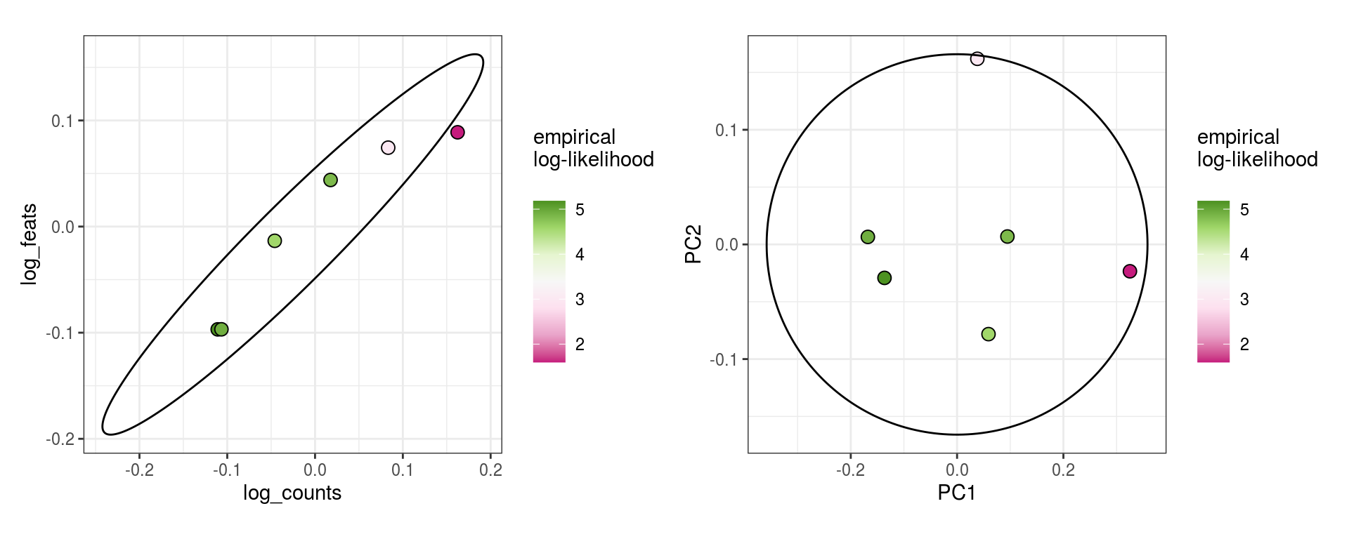
These plots show the same \(\alpha_j\) values, but as biaxials, and equivalently for PCA projections.
\(\alpha_j\) PCA values
for (i in 1:n_clusters) {
cat('### ', cluster_names[i], ' feats\n')
print(plot_alpha_js(em_list[[i]], qc_idx=1:2, pc_idx=1:2))
cat('\n\n')
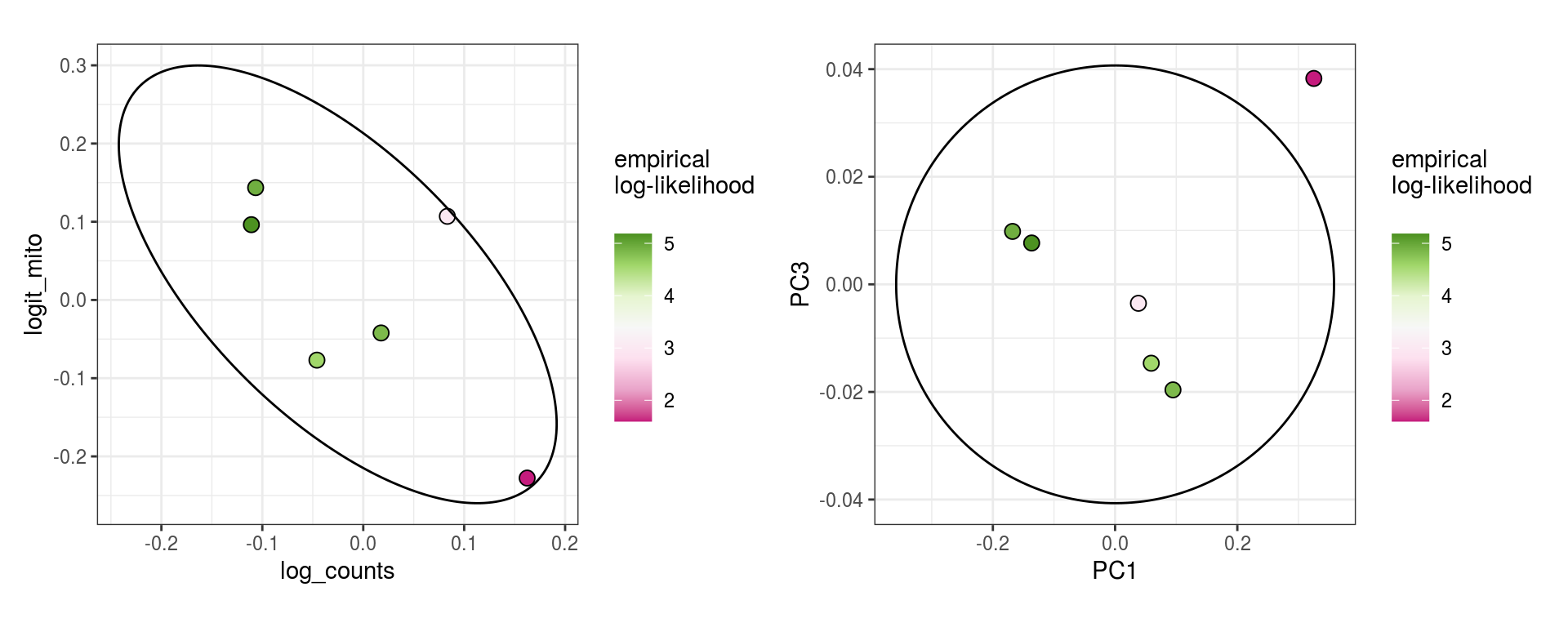
cat('### ', cluster_names[i], ' mito\n')
print(plot_alpha_js(em_list[[i]], qc_idx=c(1,3), pc_idx=c(1,3)))
cat('\n\n')
}
All mito
| Version | Author | Date |
|---|---|---|
| 1230f08 | khembach | 2020-05-27 |
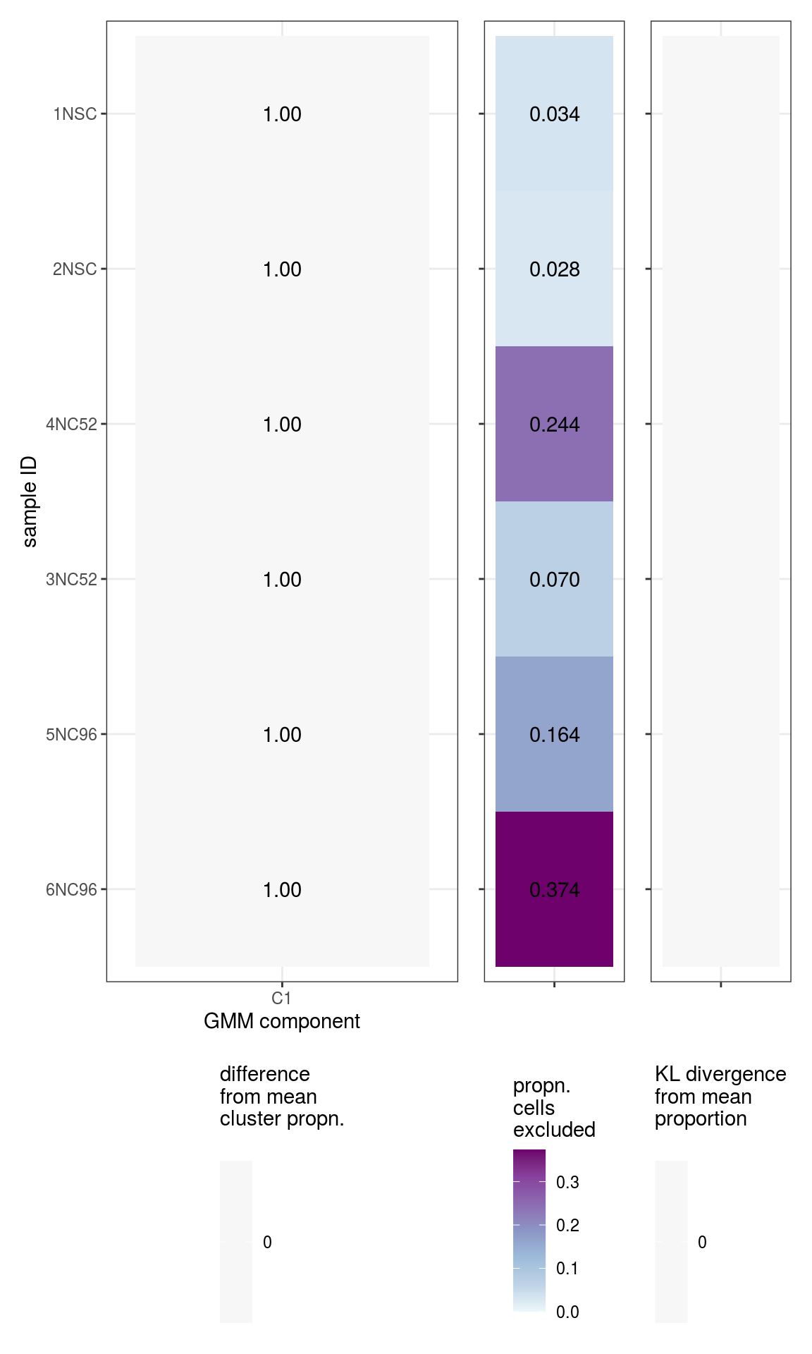
These plots show the composition of each sample in terms of the \(K\) different mixture components, plus outliers.
\(\beta_k\) values
# plot likelihoods
for (i in 1:n_clusters) {
    cat('### ', cluster_names[i], '\n')
    print(plot_beta_ks(em_list[[i]]))
    cat('\n\n')
}
All
| Version | Author | Date |
|---|---|---|
| 1230f08 | khembach | 2020-05-27 |
sessionInfo()R version 4.0.0 (2020-04-24)
Platform: x86_64-pc-linux-gnu (64-bit)
Running under: Ubuntu 16.04.6 LTS
Matrix products: default
BLAS: /usr/local/R/R-4.0.0/lib/libRblas.so
LAPACK: /usr/local/R/R-4.0.0/lib/libRlapack.so
locale:
[1] LC_CTYPE=en_US.UTF-8 LC_NUMERIC=C
[3] LC_TIME=en_US.UTF-8 LC_COLLATE=en_US.UTF-8
[5] LC_MONETARY=en_US.UTF-8 LC_MESSAGES=en_US.UTF-8
[7] LC_PAPER=en_US.UTF-8 LC_NAME=C
[9] LC_ADDRESS=C LC_TELEPHONE=C
[11] LC_MEASUREMENT=en_US.UTF-8 LC_IDENTIFICATION=C
attached base packages:
[1] parallel stats4 stats graphics grDevices utils datasets
[8] methods base
other attached packages:
[1] SingleCellExperiment_1.10.1 SummarizedExperiment_1.18.1
[3] DelayedArray_0.14.0 matrixStats_0.56.0
[5] Biobase_2.48.0 GenomicRanges_1.40.0
[7] GenomeInfoDb_1.24.0 IRanges_2.22.2
[9] S4Vectors_0.26.1 BiocGenerics_0.34.0
[11] patchwork_1.0.0 dplyr_0.8.5
[13] SampleQC_0.1.1 workflowr_1.6.2
loaded via a namespace (and not attached):
[1] mclust_5.4.6 Rcpp_1.0.4.6 lattice_0.20-41
[4] assertthat_0.2.1 rprojroot_1.3-2 digest_0.6.25
[7] RSpectra_0.16-0 R6_2.4.1 backports_1.1.7
[10] evaluate_0.14 ggplot2_3.3.0 pillar_1.4.4
[13] zlibbioc_1.34.0 rlang_0.4.6 data.table_1.12.8
[16] kernlab_0.9-29 whisker_0.4 mvnfast_0.2.5
[19] Matrix_1.2-18 rmarkdown_2.1 labeling_0.3
[22] splines_4.0.0 stringr_1.4.0 mixtools_1.2.0
[25] uwot_0.1.8 igraph_1.2.5 RCurl_1.98-1.2
[28] munsell_0.5.0 compiler_4.0.0 httpuv_1.5.2
[31] xfun_0.14 pkgconfig_2.0.3 segmented_1.1-0
[34] htmltools_0.4.0 tidyselect_1.1.0 tibble_3.0.1
[37] GenomeInfoDbData_1.2.3 codetools_0.2-16 crayon_1.3.4
[40] later_1.0.0 MASS_7.3-51.6 bitops_1.0-6
[43] grid_4.0.0 gtable_0.3.0 lifecycle_0.2.0
[46] git2r_0.27.1 magrittr_1.5 scales_1.1.1
[49] stringi_1.4.6 farver_2.0.3 XVector_0.28.0
[52] fs_1.4.1 promises_1.1.0 ellipsis_0.3.1
[55] vctrs_0.3.0 BiocStyle_2.16.0 RColorBrewer_1.1-2
[58] tools_4.0.0 forcats_0.5.0 glue_1.4.1
[61] purrr_0.3.4 survival_3.1-12 yaml_2.2.1
[64] colorspace_1.4-1 BiocManager_1.30.10 knitr_1.28