Preprocessing and QC
Katharina Hembach
5/25/2020
Last updated: 2020-06-17
Checks: 7 0
Knit directory: neural_scRNAseq/
This reproducible R Markdown analysis was created with workflowr (version 1.6.2). The Checks tab describes the reproducibility checks that were applied when the results were created. The Past versions tab lists the development history.
Great! Since the R Markdown file has been committed to the Git repository, you know the exact version of the code that produced these results.
Great job! The global environment was empty. Objects defined in the global environment can affect the analysis in your R Markdown file in unknown ways. For reproduciblity it’s best to always run the code in an empty environment.
The command set.seed(20200522) was run prior to running the code in the R Markdown file. Setting a seed ensures that any results that rely on randomness, e.g. subsampling or permutations, are reproducible.
Great job! Recording the operating system, R version, and package versions is critical for reproducibility.
Nice! There were no cached chunks for this analysis, so you can be confident that you successfully produced the results during this run.
Great job! Using relative paths to the files within your workflowr project makes it easier to run your code on other machines.
Great! You are using Git for version control. Tracking code development and connecting the code version to the results is critical for reproducibility.
The results in this page were generated with repository version 7379a9b. See the Past versions tab to see a history of the changes made to the R Markdown and HTML files.
Note that you need to be careful to ensure that all relevant files for the analysis have been committed to Git prior to generating the results (you can use wflow_publish or wflow_git_commit). workflowr only checks the R Markdown file, but you know if there are other scripts or data files that it depends on. Below is the status of the Git repository when the results were generated:
Ignored files:
    Ignored:    .DS_Store
    Ignored:    .Rhistory
    Ignored:    .Rproj.user/
    Ignored:    ._.DS_Store
    Ignored:    ._MA.pdf
    Ignored:    ._MA2.pdf
    Ignored:    ._MA_plots.pdf
    Ignored:    ._Rplots.pdf
    Ignored:    .__workflowr.yml
    Ignored:    ._hm.pdf
    Ignored:    ._neural_scRNAseq.Rproj
    Ignored:    ._sample5_MA_2nd_pop.pdf
    Ignored:    ._sample5_QC_2nd_pop.pdf
    Ignored:    ._tmp.pdf
    Ignored:    ._tmp_detected.pdf
    Ignored:    ._tmp_manual_discard.pdf
    Ignored:    ._tmp_manual_discard1.pdf
    Ignored:    ._tmp_manual_discard_all.pdf
    Ignored:    ._tmp_manual_discard_all1.pdf
    Ignored:    analysis/.DS_Store
    Ignored:    analysis/.Rhistory
    Ignored:    analysis/._.DS_Store
    Ignored:    analysis/._01-preprocessing.Rmd
    Ignored:    analysis/._01-preprocessing.html
    Ignored:    analysis/._02.1-SampleQC.Rmd
    Ignored:    analysis/._04-clustering.Rmd
    Ignored:    analysis/._04-clustering.knit.md
    Ignored:    analysis/._05-annotation.Rmd
    Ignored:    analysis/.__site.yml
    Ignored:    analysis/._additional_filtering.Rmd
    Ignored:    analysis/._additional_filtering_clustering.Rmd
    Ignored:    analysis/02-1-SampleQC_cache/
    Ignored:    analysis/02-quality_control_cache/
    Ignored:    analysis/02.1-SampleQC_cache/
    Ignored:    analysis/03-filtering_cache/
    Ignored:    analysis/04-clustering_cache/
    Ignored:    analysis/05-annotation_cache/
    Ignored:    analysis/additional_filtering_cache/
    Ignored:    analysis/additional_filtering_clustering_cache/
    Ignored:    analysis/sample5_QC_cache/
    Ignored:    data/.DS_Store
    Ignored:    data/._.DS_Store
    Ignored:    data/._.smbdeleteAAA17ed8b4b
    Ignored:    data/._metadata.csv
    Ignored:    data/data_sushi/
    Ignored:    data/filtered_feature_matrices/
    Ignored:    output/.DS_Store
    Ignored:    output/._.DS_Store
    Ignored:    output/additional_filtering.rds
    Ignored:    output/figures/
    Ignored:    output/sce_01_preprocessing.rds
    Ignored:    output/sce_02_quality_control.rds
    Ignored:    output/sce_03_filtering.rds
    Ignored:    output/sce_preprocessing.rds
    Ignored:    output/so_04_clustering.rds
    Ignored:    output/so_additional_filtering_clustering.rds

Untracked files:
    Untracked:  MA.pdf
    Untracked:  MA2.pdf
    Untracked:  MA_plots.pdf
    Untracked:  Rplots.pdf
    Untracked:  analysis/additional_filtering.Rmd
    Untracked:  analysis/additional_filtering_clustering.Rmd
    Untracked:  analysis/sample5_QC.Rmd
    Untracked:  analysis/tabsets.Rmd
    Untracked:  hm.pdf
    Untracked:  sample5_MA_2nd_pop.pdf
    Untracked:  sample5_QC_2nd_pop.pdf
    Untracked:  scripts/
    Untracked:  tmp.pdf
    Untracked:  tmp_detected.pdf
    Untracked:  tmp_manual_discard.pdf
    Untracked:  tmp_manual_discard1.pdf
    Untracked:  tmp_manual_discard_all.pdf
    Untracked:  tmp_manual_discard_all1.pdf

Unstaged changes:
    Modified:   analysis/_site.yml
Note that any generated files, e.g. HTML, png, CSS, etc., are not included in this status report because it is ok for generated content to have uncommitted changes.
These are the previous versions of the repository in which changes were made to the R Markdown (analysis/01-preprocessing.Rmd) and HTML (docs/01-preprocessing.html) files. If you’ve configured a remote Git repository (see ?wflow_git_remote), click on the hyperlinks in the table below to view the files as they were in that past version.
| File | Version | Author | Date | Message |
|---|---|---|---|---|
| Rmd | 7379a9b | khembach | 2020-06-17 | add histo and PCA for scDblFinder results |
| html | 7e96c71 | khembach | 2020-06-17 | Build site. |
| Rmd | 336ee0c | khembach | 2020-06-17 | wflow_publish(“analysis/01-preprocessing.Rmd”, verbose = TRUE, |
| html | f3c8307 | khembach | 2020-06-08 | Build site. |
| Rmd | 013c877 | khembach | 2020-06-08 | use filtered feature matrix of sample 3 and 5 |
| html | 1230f08 | khembach | 2020-05-27 | Build site. |
| Rmd | 6be1a5a | khembach | 2020-05-27 | rebuild without cache and SampleQC report |
| html | d56ccca | khembach | 2020-05-26 | Build site. |
| Rmd | 24db792 | khembach | 2020-05-26 | Preprocessing and quality control plots |
Load packages
library(DropletUtils)
library(scDblFinder)
library(BiocParallel)
library(ggplot2)
library(scater)
Importing CellRanger output and metadata
fs <- dir(path = "data/filtered_feature_matrices",
                pattern = "^[1-6]N*", recursive = FALSE, full.names = TRUE)
names(fs) <- basename(fs)
## we want to analyse the count matrix
fs <- sapply(fs, function(x) file.path(x, "filtered_feature_bc_matrix.h5"))
sce <- read10xCounts(samples = fs)

# rename colnames and dimnames
rowData(sce)$Type <- NULL
names(rowData(sce)) <- c("ensembl_id", "symbol")
names(colData(sce)) <- c("sample_id", "barcode")
sce$sample_id <- factor(sce$sample_id)
dimnames(sce) <- list(with(rowData(sce), paste(ensembl_id, symbol, sep = ".")),
                      with(colData(sce), paste(barcode, sample_id, sep = ".")))

# load metadata
meta <- read.csv(file.path("data", "metadata.csv"))
m <- match(sce$sample_id, meta$sample)
sce$group_id <- meta$group[m]
Remove undetected genes and doublets
sce <- sce[rowSums(counts(sce) > 0) > 0, ]
dim(sce)
[1] 19375 52830# doublet detection with 'scDblFinder'
# the expected proportion of doublets is 1% per 1000 cells
sce <- scDblFinder(sce, samples="sample_id", BPPARAM=MulticoreParam(6))
table(colData(sce)[,c("scDblFinder.class", "sample_id")]) sample_id
scDblFinder.class 1NSC 2NSC 3NC52 4NC52 5NC96 6NC96
doublet 838 813 904 826 422 404
singlet 8908 8860 9096 8889 6578 6292# histogram of the doublet scores
dat <- as.data.frame(colData(sce)[c("scDblFinder.score",
"scDblFinder.class", "sample_id")])
dat$scDblFinder.class <- factor(dat$scDblFinder.class,
levels = c("singlet", "doublet"))
p <- ggplot(dat, aes(scDblFinder.score)) +
geom_histogram(bins = 100) +
facet_grid(vars(sample_id), vars(scDblFinder.class)) +
scale_y_log10()
print(p)Warning: Transformation introduced infinite values in continuous y-axisWarning: Removed 625 rows containing missing values (geom_bar).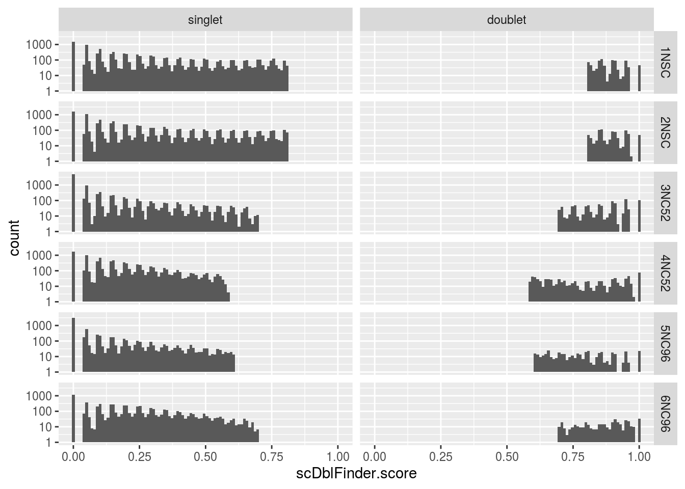
| Version | Author | Date |
|---|---|---|
| 7e96c71 | khembach | 2020-06-17 |
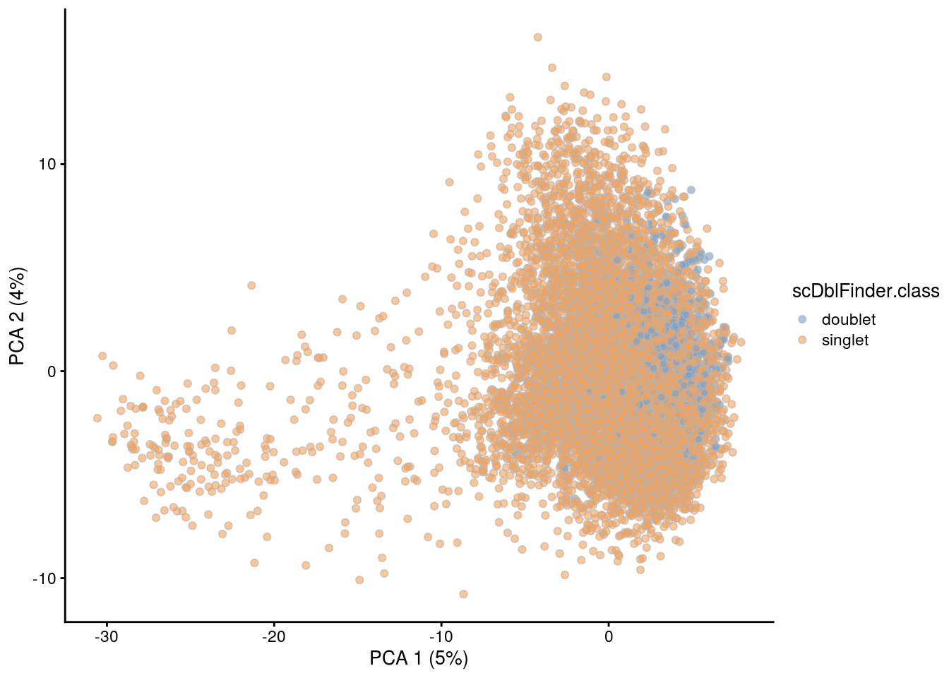
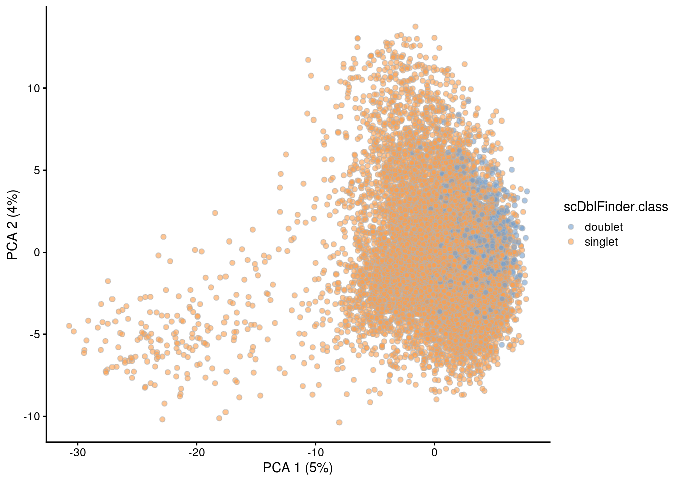
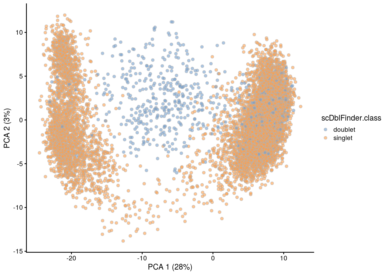
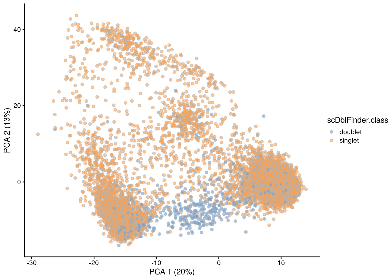
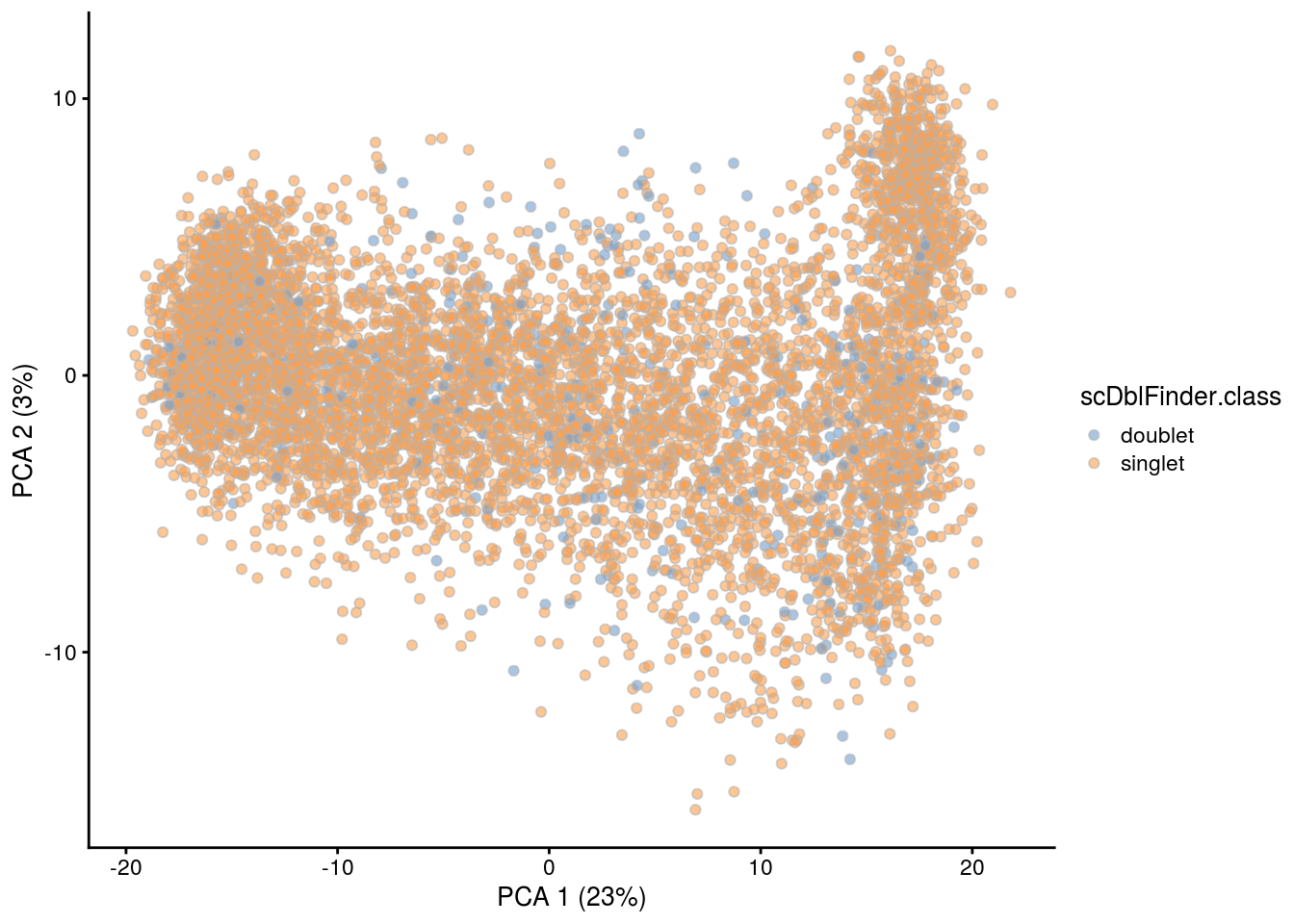
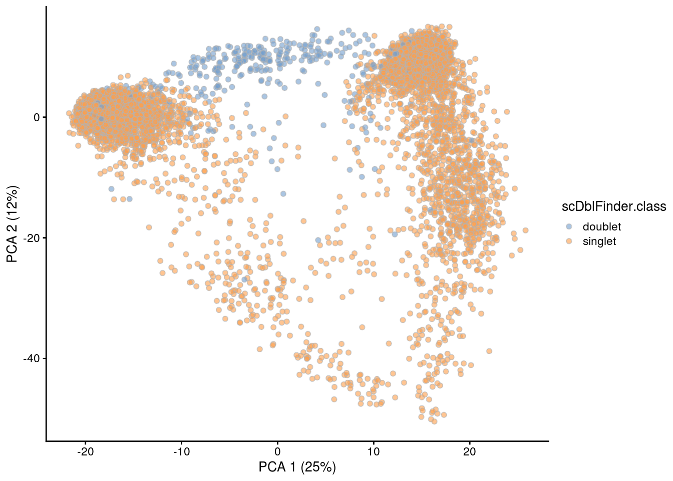
## PCA plot colored by doublet score
for (i in levels(sce$sample_id)) {
  print(i)
  subs <- sce[,sce$sample_id == i]
  subs <- logNormCounts(subs)
  subs <- runPCA(subs)
  print(plotPCA(subs, colour_by = "scDblFinder.score"))
  print(plotPCA(subs, colour_by = "scDblFinder.class"))
}
[1] "1NSC"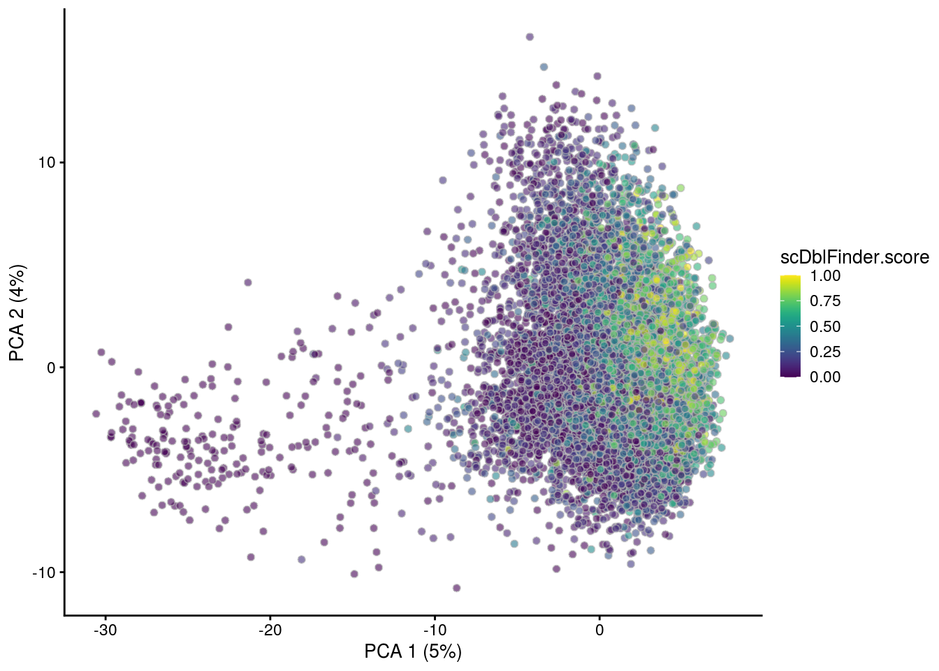
[1] "2NSC"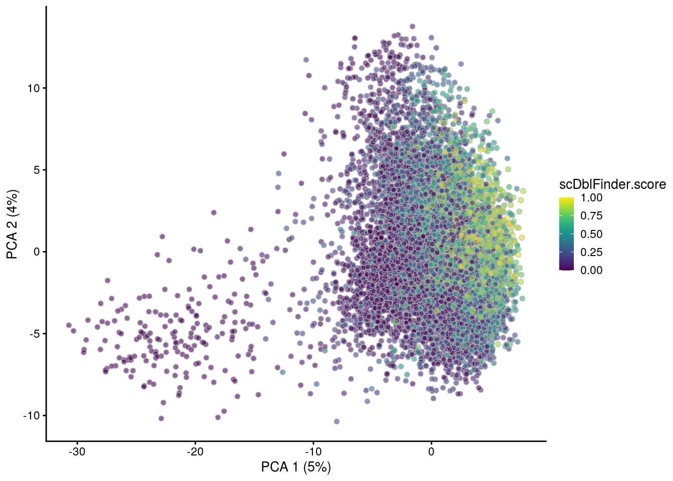
[1] "3NC52"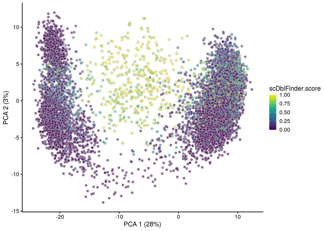
[1] "4NC52"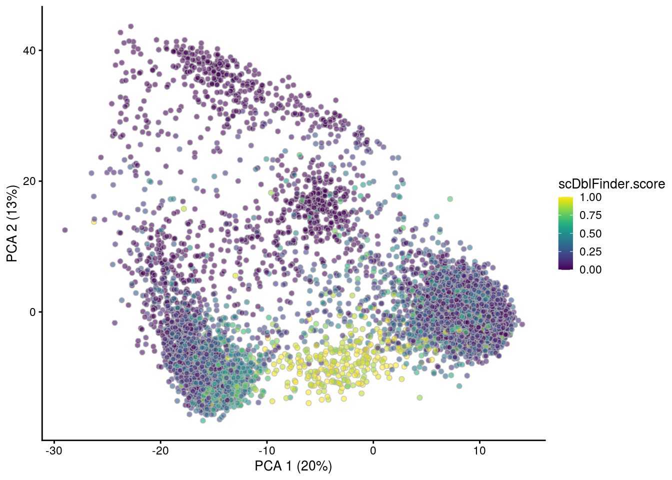
[1] "5NC96"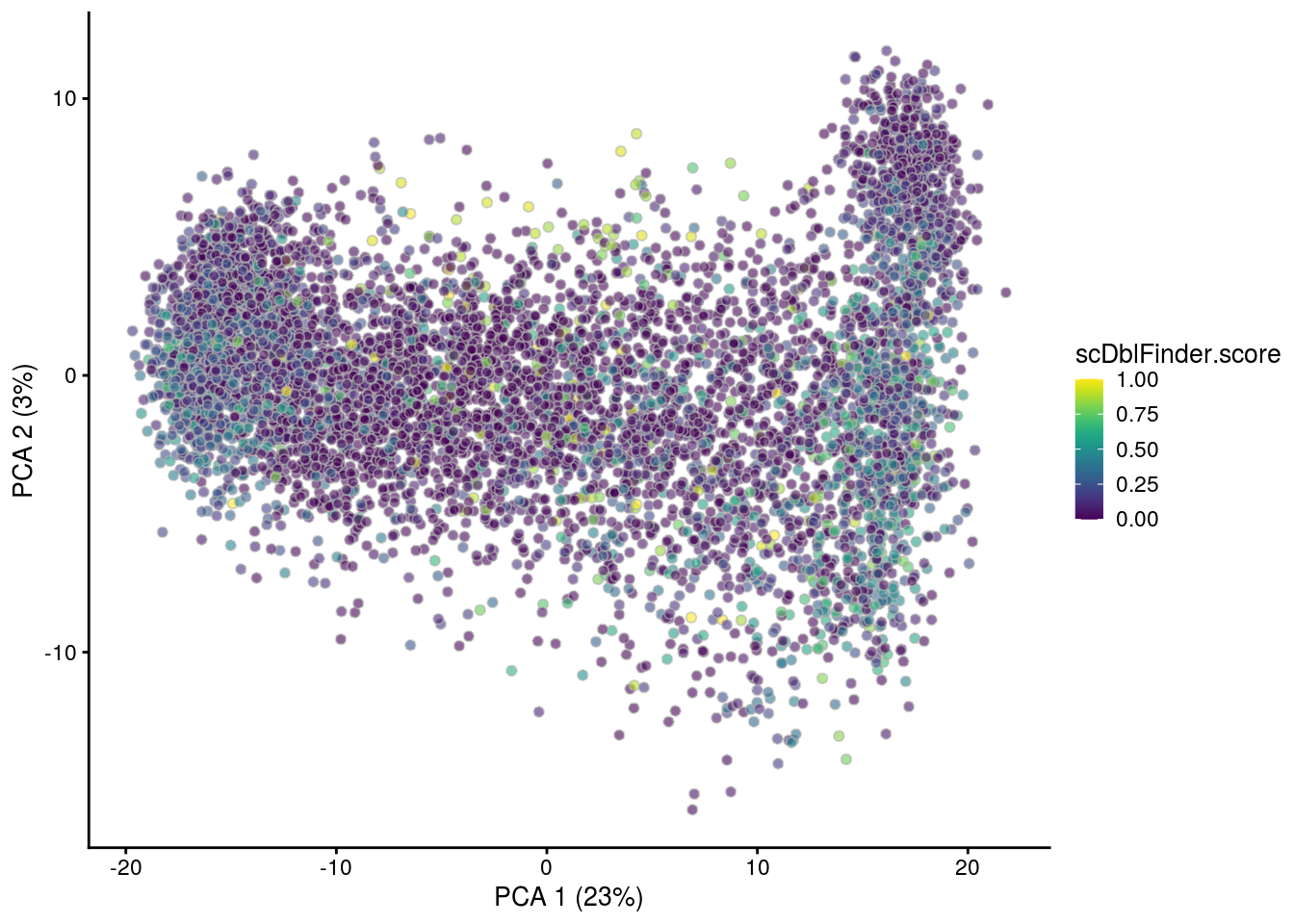
[1] "6NC96"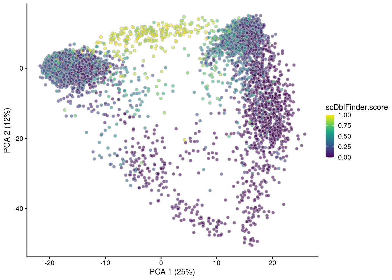
# we remove the cells that were classified as doublets
sce <- sce[,sce$scDblFinder.class == "singlet"]
Save data to RDS
saveRDS(sce, file.path("output", "sce_01_preprocessing.rds"))
sessionInfo()R version 4.0.0 (2020-04-24)
Platform: x86_64-pc-linux-gnu (64-bit)
Running under: Ubuntu 16.04.6 LTS
Matrix products: default
BLAS: /usr/local/R/R-4.0.0/lib/libRblas.so
LAPACK: /usr/local/R/R-4.0.0/lib/libRlapack.so
locale:
[1] LC_CTYPE=en_US.UTF-8 LC_NUMERIC=C
[3] LC_TIME=en_US.UTF-8 LC_COLLATE=en_US.UTF-8
[5] LC_MONETARY=en_US.UTF-8 LC_MESSAGES=en_US.UTF-8
[7] LC_PAPER=en_US.UTF-8 LC_NAME=C
[9] LC_ADDRESS=C LC_TELEPHONE=C
[11] LC_MEASUREMENT=en_US.UTF-8 LC_IDENTIFICATION=C
attached base packages:
[1] parallel stats4 stats graphics grDevices utils datasets
[8] methods base
other attached packages:
[1] scater_1.16.0 ggplot2_3.3.0
[3] BiocParallel_1.22.0 scDblFinder_1.1.15
[5] DropletUtils_1.8.0 SingleCellExperiment_1.10.1
[7] SummarizedExperiment_1.18.1 DelayedArray_0.14.0
[9] matrixStats_0.56.0 Biobase_2.48.0
[11] GenomicRanges_1.40.0 GenomeInfoDb_1.24.0
[13] IRanges_2.22.2 S4Vectors_0.26.1
[15] BiocGenerics_0.34.0 workflowr_1.6.2
loaded via a namespace (and not attached):
[1] viridis_0.5.1 edgeR_3.30.0
[3] BiocSingular_1.4.0 viridisLite_0.3.0
[5] DelayedMatrixStats_1.10.0 R.utils_2.9.2
[7] assertthat_0.2.1 statmod_1.4.34
[9] dqrng_0.2.1 vipor_0.4.5
[11] GenomeInfoDbData_1.2.3 yaml_2.2.1
[13] pillar_1.4.4 backports_1.1.7
[15] lattice_0.20-41 glue_1.4.1
[17] limma_3.44.1 digest_0.6.25
[19] promises_1.1.0 XVector_0.28.0
[21] randomForest_4.6-14 colorspace_1.4-1
[23] cowplot_1.0.0 htmltools_0.4.0
[25] httpuv_1.5.2 Matrix_1.2-18
[27] R.oo_1.23.0 pkgconfig_2.0.3
[29] zlibbioc_1.34.0 purrr_0.3.4
[31] scales_1.1.1 HDF5Array_1.16.0
[33] whisker_0.4 later_1.0.0
[35] git2r_0.27.1 tibble_3.0.1
[37] farver_2.0.3 ellipsis_0.3.1
[39] withr_2.2.0 magrittr_1.5
[41] crayon_1.3.4 evaluate_0.14
[43] R.methodsS3_1.8.0 fs_1.4.1
[45] beeswarm_0.2.3 tools_4.0.0
[47] data.table_1.12.8 lifecycle_0.2.0
[49] stringr_1.4.0 Rhdf5lib_1.10.0
[51] munsell_0.5.0 locfit_1.5-9.4
[53] irlba_2.3.3 compiler_4.0.0
[55] rsvd_1.0.3 rlang_0.4.6
[57] rhdf5_2.32.0 grid_4.0.0
[59] RCurl_1.98-1.2 BiocNeighbors_1.6.0
[61] igraph_1.2.5 labeling_0.3
[63] bitops_1.0-6 rmarkdown_2.1
[65] codetools_0.2-16 gtable_0.3.0
[67] R6_2.4.1 gridExtra_2.3
[69] knitr_1.28 dplyr_0.8.5
[71] rprojroot_1.3-2 stringi_1.4.6
[73] ggbeeswarm_0.6.0 Rcpp_1.0.4.6
[75] scran_1.16.0 vctrs_0.3.0
[77] tidyselect_1.1.0 xfun_0.14